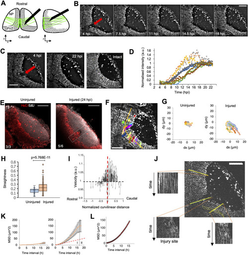
Optic tectum wound closes within 24 h after the injury.

(A) Organisation of neurons in the optic tectum and our injury model. Neurons (dark circles), surrounded by astrocytic processes (green), are arranged in layers (lamina, dashed lines) and columns as shown in XY and XZ sections; an insect pin (black) is used to injure the optic tectum down to the periventricular zone. NP: neuropil, PVZ: periventricular zone. (B) Time series of Tg(h2a:GFP) 4 dpf larvae after an injury showing wound closure (red arrow indicates wound position). (C) Wound closure between 4 hpi (left) and 22 hpi (middle) shows the restoration of the tissue as compared to the intact tectum (right; red arrow indicates wound position). (D) Variation over time of the fluorescence intensity inside the injury site during tectum repair (n = 11 larvae). (E) EdU staining (white) and HuC immunofluorescence (red) in uninjured Tg(h2a:GFP) larvae (left) and injured Tg(h2a:GFP) larvae (right). (F) Individual trajectories of neuron nuclei in the tectum of injured Tg(h2a:GFP) 4 dpf larvae (coloured traces). The starting points of individual trajectories were projected perpendicularly (white lines) on the curved rostrocaudal extend (orange curve). (G) Individual trajectories in uninjured and injured larvae showed an increased and directional XY displacement for injured animals. (H) Straightness analysis of uninjured (n = 7) and injured (n = 11) larvae showing that trajectories of neuronal nuclei are more elongated after injury. Box plots show the median, box edges represent the 25th and 75th percentiles, and whiskers indicate ± 1.5 x the interquartile range. (P <0.0001, t test). (I) Trajectory directionality analysis of individual nuclei after rostrocaudal curve linearisation indicates trajectory anisotropy. The injury centre position is represented by the dashed red line. (J) Kymographs at different locations in the PVZ area of an injured fish show that neurons keep their laminar organisation over time. (K) Mean-squared displacement (MSD) analysis of individual trajectories of neuronal cell nuclei for uninjured (left) and injured (right) larvae shows two phases of displacement: I, a superdiffusive behaviour after injury; and II, a slower increase compatible with diffusion. The red dashed line shows the MSD for a diffusive case. (D, L) MSD superdiffusion model, MSD(t) Ã t—fit of the experimental MSD curve in (D). Blue curve: theoretical model; red points: experimental values. R > 0.999, — = 1.86. All images are oriented with the rostral side up. Scale bars represent 50 μm on all images.

Optic tectum wounds close via tissue deformation.

(A) Fluorescence images of a Tg(her4.3:GFP-F); Tg(elavl3:MA-mKate2) fish at 4 dpf. (B) Measurement of the neuropil contour deformation using Tg(her4.3:GFP-F); Tg(elavl3:MA-mKate2) larvae. Deformation is measured along the axes shown (orange arrows). (B, C) Boxplot representation of the neuropil contour deformation measured in (B) (n = 6), represented on the caudal (y-axis, CDy, blue) and rostral (x-axis, RDx, orange) axes. (D) Deformation quantification using the PVZ boundary in Tg(h2a:GFP) larvae. (D, E) Boxplot representation of the deformation measurements as performed in (D) (n = 6). (F) Model of viscoelastic dynamics of neuron displacement comprising three phases (see Supplemental Information). (G) Example of experimental wound closure curve (black dots) fitted by the model (red curve). (H) Example images of injured optic tectum of control and blebbistatin-treated Tg(Xla.Tubb:DsRed) animals at 7 and 24 hpi. The orange dashed lines show the position of the injury. The white dashed lines show the analysis regions for calculating the repair index. (I) Quantification of the repair index (RI) for control (n = 9) and blebbistatin-treated (n = 12) fish. t test, P < 0.05. Box plots show the median, box edges represent the 25th and 75th percentiles, and whiskers show the full data range. Scale bars represent 50 μm on all images. All quantifications are between 4 and 24 hpi unless otherwise stated.

Microglial invasion in the neuropil correlates with the kinetics of wound closure.

(A) Displacement field analysis showing the direction of displacement of individual neuronal nuclei (black arrows). The orange lines show how the intersection points (black spots) between trajectories are estimated. (B) Polar representation (in degrees) of the position of intersection points of individual trajectories of neuronal nuclei from 10 animals after tectum size normalisation and rotation. The optic tectum is represented as an overlay (boundaries in dark grey and PVZ in light grey). (C) Accumulation of cells in the neuropil (inside the orange circle) after injury in Tg(h2a:GFP) larvae at 20 hpi. (D) Identification of the accumulated cells as mpeg1+ cells using Tg(mpeg1:mCherry) (red) larvae, combined with nuclear staining (Hoechst 33342, grey). (E) Identification of the mpeg1:GFP+ cells as microglia using 4C4 immunofluorescence in an injured Tg(Xla.Tubb:DsRed); Tg(mpeg1:GFP) fish. White arrows point out mpeg1:GFP+/4C4+ double-labelled cells. (F) Polar representation of microglial positions (N = 308 from 15 animals, magenta) in the neuropil compared with intersection points of trajectories of neuronal nuclei (black, green spots: centre of gravity of intersection points for each animal). (G) Selected frames of a time-lapse imaging series of an injured Tg(Xla.Tubb:DsRed); Tg(mpeg1:GFP) transgenic animal show the recruitment and accumulation of microglia in the injury site. (H) Lower magnification image of an injured Tg(Xla.Tubb:DsRed); Tg(mpeg1:GFP) transgenic animal showing that microglia did not accumulate in the intact contralateral tectum. (I) Kinetics of microglial accumulation from 2 hpi to 13 hpi (black square) and the average wound closure kinetics (black dots). (J) Dual-channel single-cell tracking of neuronal cell bodies (left, red trajectories) and microglia (right, green trajectories) in an injured Tg(Xla.Tubb:DsRed); Tg(mpeg1:GFP) larva. (K) Boxplot representation of the discrete Fréchet distance estimation between microglial trajectories and experimental (orange) and randomised (blue) trajectories of neuronal cell nuclei. Box plots show the median, box edges represent the 25th and 75th percentiles, and whiskers show ± 1.5 x the interquartile range. t test, P <0.05. Scale bars represent 50 μm on all images.

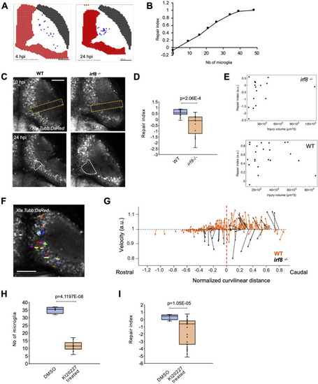
Microglia are necessary for brain tissue repair.

(A) Example of simulation result showing microglia accumulation and wound closure. Left: simulated tissue after injury with patches of microglia agents in the neuropil. Right: the same simulation at 24 hpi. (B) Relation between the repair index estimated on the simulated data and the number of microglia agents in the simulation. (C) Images of an injured tectum in WT and irf8–/– Tg(Xla.Tubb:DsRed) larvae, right after the injury (0 hpi) and at 24 hpi. The orange dashed lines show where the injury was made. The white dashed lines show the analysis regions for calculating the repair index. Scale bar: 20 µm. (D) Quantification of the repair index (=1 - V@24 hpi/V@4 hpi) in WT (n = 21) and ifr8 mutant larvae (n = 17). t test P-value <0.001. (E) Correlation analysis of the repair index versus initial injury volume shows that the repair index is independent of the initial size of the injury. (F) Trajectories of neuronal cell bodies in an injured irf8 mutants (Scale bar: 50 µm). (G) Comparison of anisotropy of trajectories in WT (orange, from Fig 1I) and in ifr8 mutants (black). (H) Quantification of the depletion of microglia using KI20227 t test P-value <0.0001 (Controls n = 4, treated n = 10). (I) Measurement of the repair index in control (n = 12) and KI20227 treated (n = 26) animals. t test P-value <0.0001. Box plots show the median, box edges represent the 25th and 75th percentiles, and whiskers show the full data range. Scale bars represent 50 µm on all images.

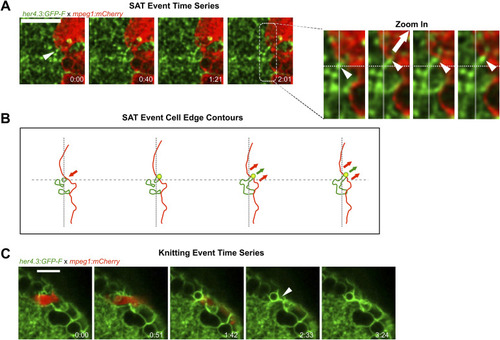
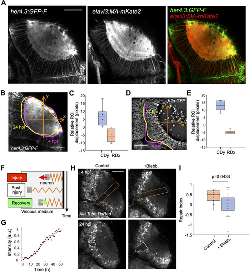
Microglial contacts displace astrocytic processes.

(A) Fast time-lapse imaging sequence on a Tg(her4.3:GFP-F);Tg(mpeg1:mCherry) larva showing an SAT process. The white arrow points out the adhesion event. (A′) Cropped sequence from (A). The small white arrows point to astrocytic protrusion pulled by microglia protrusion. The big arrow shows the direction of the traction force. The dashed line indicates the initial and final positions. (A, B) Outline of microglia (red) and astrocytic structures (green) from images in (A). Arrows show the direction of displacement. (C) Example of a knitting event. All scale bars: 10.

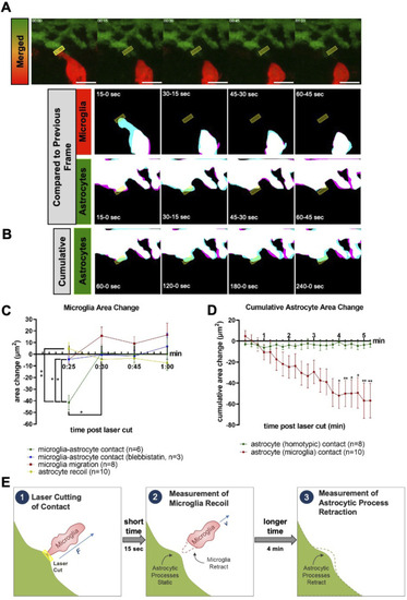
Microglia and astrocytic process recoil after laser severance of contact sites.

(A) Diagram of laser-induced microglial recoil away from astrocytic contacts and slower retraction of astrocytic processes. (B) Time-lapse images of microglia (red) and astrocytes (green) after laser ablation (upper, up to 1 min post-ablation), with area masks overlaid between adjacent time points for microglia (middle) and astrocytes (lower). (C) Cumulative area masks of astrocytes for 1–4 min post-ablation. (B, D) Change in area after laser ablation for microglia that were contacting astrocytes (green, n = 6), blebbistatin-treated microglia contacting astrocytes (blue, n = 3), microglial migration (red, n = 8), and astrocytes that were contacting microglia (yellow, n = 10). Area change represents the difference between T(n + 1) and Tn as shown in (B) as magenta and blue, respectively. (E) Cumulative area change for astrocytes with homotypic (green, n = 8) or microglial (red, n = 6) contacts after ablation. Area change represents the total area changed between T0 and the given time point. Statistics were assessed by two-way ANOVA with Šídák’s multiple comparison test, *P < 0.05, **P < 0.01. All scale bars represent 10 μm, and all ablation sites are marked with yellow boxes on montages.

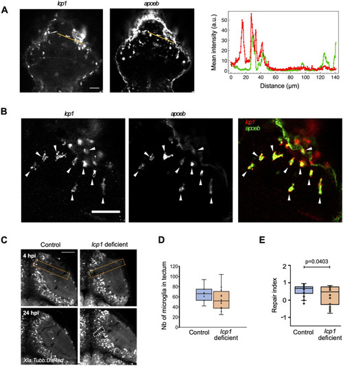
Microglial action relies on lcp1.

(A) Expression of lcp1 and apoeb as detected by hybridisation chain reaction fluorescence in situ hybridisation in injured larvae at 6 hpi. The intensity profiles shown on the graph (red: lcp1; green: apoeb) were measured along the orange lines shown in the images. (B) Zoomed-in hybridisation chain reaction fluorescence in situ hybridisation images for lcp1a (green) and apoeb (red), showing an almost complete overlap of patterns. Arrows point to lcp1+/apoeb+ cells at the lesion site. (C) Representative images of wound closure in control and haCR-injected animals are shown; orange dashed lines: injury site; white dashed lines: wound delimitation in the PVZ. (D) Boxplot representation of the repair index in all haCR-injected animals (P from an unpaired t test). (E) Boxplot representation of the number of microglia in the optic tectum at 24 hpi in haCR-injected animals. All t tests were non-significant (P > 0.05). For all experiments, n = 4 for control-injected, and n = 10 for haCR-injected animals. All scale bars represent 50 μm.

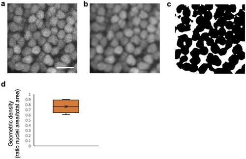
Neuronal nuclei show a dense hexagonal packing in the optic tectum.

(A) Zoom in on neuronal cell nucleus arrangement in the PVZ (scale bar: 10 μm). (B) Same image after filtering using a Gaussian blur to reduce noise before quantification is shown. (C) Thresholded binary images with nuclei in black and interstitial space in white are shown. (D) Quantification of the geometrical density of neuronal cell nuclei (n = 6). Box plots show the median, box edges represent the 25th and 75th percentiles, and whiskers show the full data range.

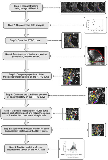
Workflow for the analysis of anisotropy of cell trajectories.

Analysis workflow used to generate the graphs in Figs 1I and 4G.

Microglial accumulation analysis workflow.

Analysis workflow used to generate the graph in Fig 3F.

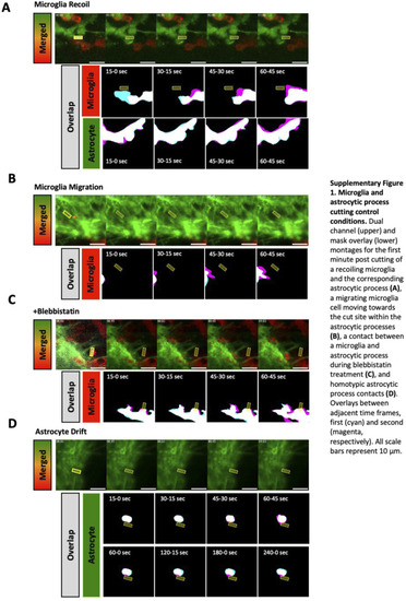
Additional examples and control conditions for cutting of microglial and astrocytic process contacts.

(A, B, C, D) Dual-channel (upper) and mask overlay (lower) montages for the first-minute post-cutting of recoiling microglia and the corresponding astrocytic process (A), a migrating microglial cell moving towards the cut site within the astrocytic processes (B), a contact between microglia and astrocytic process during blebbistatin treatment (C), and homotypic astrocytic process contacts (D). Overlays between adjacent time frames, first (cyan) and second (magenta). All scale bars represent 10 μm.

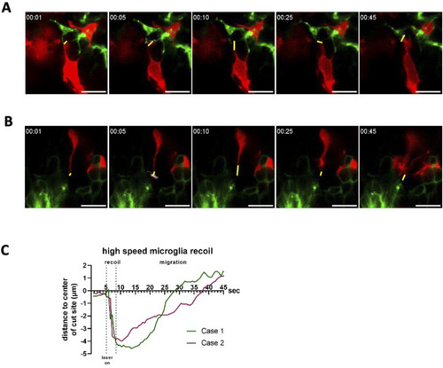
Single-plane high temporal resolution imaging of recoiling microglial contacts after laser cutting.

(A, B) Individual montages of time-lapse images of two cases of microglial retraction in response to planar cutting of contacts with astrocytic processes (A, B). The distances between the centroid of the cut site and the edge of the microglia are labelled with yellow lines. (C) Measurements of the distance between the leading edge of the microglia and the centroid of the laser cut site for each case over time (C). All scale bars represent 10 μm.

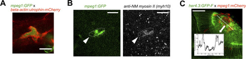
Microglia possess the molecular machinery to exert forces, and accumulation leads to increased GFAP detectability.

(A) Confocal micrograph of a microglial cell in the optic tectum, which expresses both mpeg1:GFP and beta-actin:utrophin-mCherry, illustrating that the F-actin filaments accumulate along the exterior membrane of the microglia after stab injury. (B) Microglial cell (mpeg1:GFP) immunofluorescently labelled for non-muscular myosin II, the target for blebbistatin. The cell shows notable accumulation of myosin II. (C) Horizontal section of the tectum at 12 h post-injury is shown, together with a density plot for GFP fluorescence. Astrocytic processes labelled by her4.3:GFP-F show increased fluorescence next to the accumulation of microglia in the tectal neuropil. The scale bar in (A, B) represents 10 μm.

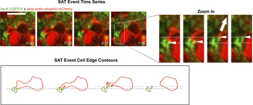
Utrophin labelling is enriched at sites of astrocyte pulling.

(Upper left) Fast time-lapse imaging sequence on a Tg(her4.3:GFP-F); Tg(beta-actin:utrophin-mCherry) larva showing an SAT process. The white arrow points out the adhesion event. (Right) Cropped sequence from upper left. White arrows point to the astrocytic node pulled by microglial protrusion. The dashed line indicates the initial position. (Lower left) Outline of microglia (red) and astrocytic structures (green) from images in the panel above. Arrows show the direction of displacement. Scale bar: 10 μm.

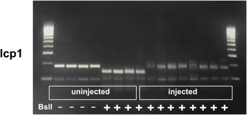
Determination of haCRs for lcp1.

Results of the RFLP technique on uninjected and injected animals for the targeted gene. Note that uninjected embryos show complete digestion with the indicated restriction enzymes, whereas haCR injection efficiently alters the enzyme recognition site and prevents digestion.