|
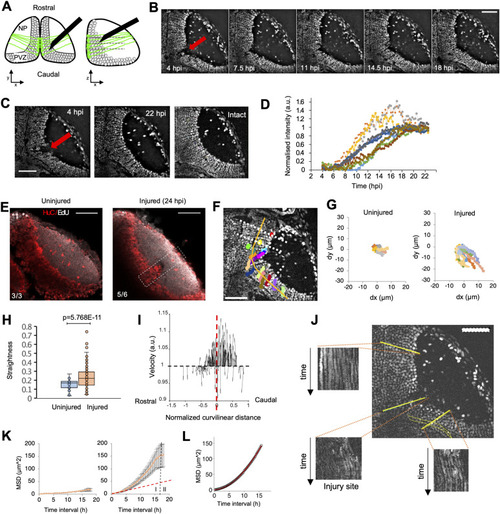
Optic tectum wound closes within 24 h after the injury. (A) Organisation of neurons in the optic tectum and our injury model. Neurons (dark circles), surrounded by astrocytic processes (green), are arranged in layers (lamina, dashed lines) and columns as shown in XY and XZ sections; an insect pin (black) is used to injure the optic tectum down to the periventricular zone. NP: neuropil, PVZ: periventricular zone. (B) Time series of Tg(h2a:GFP) 4 dpf larvae after an injury showing wound closure (red arrow indicates wound position). (C) Wound closure between 4 hpi (left) and 22 hpi (middle) shows the restoration of the tissue as compared to the intact tectum (right; red arrow indicates wound position). (D) Variation over time of the fluorescence intensity inside the injury site during tectum repair (n = 11 larvae). (E) EdU staining (white) and HuC immunofluorescence (red) in uninjured Tg(h2a:GFP) larvae (left) and injured Tg(h2a:GFP) larvae (right). (F) Individual trajectories of neuron nuclei in the tectum of injured Tg(h2a:GFP) 4 dpf larvae (coloured traces). The starting points of individual trajectories were projected perpendicularly (white lines) on the curved rostrocaudal extend (orange curve). (G) Individual trajectories in uninjured and injured larvae showed an increased and directional XY displacement for injured animals. (H) Straightness analysis of uninjured (n = 7) and injured (n = 11) larvae showing that trajectories of neuronal nuclei are more elongated after injury. Box plots show the median, box edges represent the 25th and 75th percentiles, and whiskers indicate ± 1.5 x the interquartile range. (P <0.0001, t test). (I) Trajectory directionality analysis of individual nuclei after rostrocaudal curve linearisation indicates trajectory anisotropy. The injury centre position is represented by the dashed red line. (J) Kymographs at different locations in the PVZ area of an injured fish show that neurons keep their laminar organisation over time. (K) Mean-squared displacement (MSD) analysis of individual trajectories of neuronal cell nuclei for uninjured (left) and injured (right) larvae shows two phases of displacement: I, a superdiffusive behaviour after injury; and II, a slower increase compatible with diffusion. The red dashed line shows the MSD for a diffusive case. (D, L) MSD superdiffusion model, MSD(t) Ã t—fit of the experimental MSD curve in (D). Blue curve: theoretical model; red points: experimental values. R > 0.999, — = 1.86. All images are oriented with the rostral side up. Scale bars represent 50 μm on all images.
|