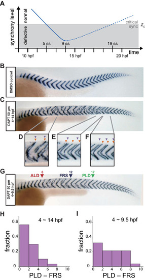
(A) Schematic time series of synchrony level during desynchronization and resynchronization. In the presence of DAPT, the synchrony level decreases due to the loss of Delta-Notch signaling (solid line). DAPT is washed out at 14 hr post-fertilization (hpf; ~9 somite stage; ss) in this panel and resynchronization starts from that time point (dotted line). If the synchrony level is higher (lower) than a critical value Zc, normal (defective) segments are formed. (B) Wild-type control embryo treated with DMSO. (C) Embryo with late DAPT washout at 14 hpf (9 ss). Enlargements of (D) broken or fragmented boundaries, (E) incorrect number of boundaries and (F) left-right misaligned boundaries are shown below. (G) Embryo with early DAPT washout at 9.5 hpf (0 ss). Red, blue and green triangles indicate the anterior limit of defect (ALD), first recovered segment (FRS) and posterior limit of defect (PLD), respectively. (H), (I) Histograms of the difference between PLD and FRS (PLD ? FRS) for embryos with DAPT washout at (H) late (14 hpf; n = 30) and (I) early (9.5 hpf; n = 28) stages. Numbers of embryos examined in (H) and (I) were 15 and 14, respectively. FRS and PLD were measured separately between left and right sides of embryos. p<0.05 in Kolmogorov-Smirnov test.

(A) Segment defects and definitions of the anterior limit of defects (ALD), first recovered segment (FRS) and posterior limit of defects (PLD). Blue chevrons indicate segment boundaries. Fragmented or broken chevrons represent defective boundaries. Only one embryonic side is illustrated. In this study, embryos were scored one side at a time. Distributions of defective segments may be different between left and right sides of embryos. ALD and PLD is defined with the posterior boundary of the first and last defective segments, respectively. FRS is defined with the anterior boundary of the first normal segment. (B) Spatial distribution of defective segment boundaries for DAPT washout at 9.5 hr post fertilization (hpf) (0 somite-stage, ss: triangles, n = 28) and at 14 hpf (9 ss: crosses, n = 30). The horizontal axis is segment boundary number. The vertical axis is the fraction of defective segment boundaries over embryos. Because of the increase in the fraction of defective segments, the desynchronization phase is considered to continue until segment 9. The two inverted triangles indicate DAPT washout times. (C)-(G) Left: Histograms of the difference between FRS and PLD (PLD – FRS). When the first normal segment boundary is found immediately after the last defective boundary, FRS and PLD coincide, and PLD – FRS is zero, see (A) and Materials and methods. Right: FRS and PLD for each embryonic left-right side. The left circles indicate FRS. The right circles connected with the left circles by lines indicate PLD of the same embryonic side. Single circles indicate that FRS and PLD are the same. The number of examined embryonic left-right sides is shown in the vertical axis. DAPT washout at (C) 9.5 hpf, (D) 11 hpf, (E) 12.5 hpf, (F) 14 hpf, and (G) 15.5 hpf.

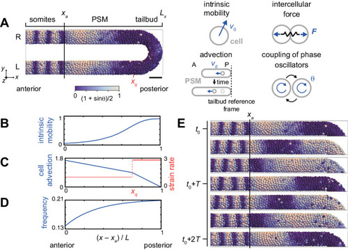
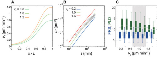
(A) U-shape geometry of the PSM and tailbud (left), and schematics of key ingredients in the model (right). Each sphere represents a PSM cell. The scale bar indicates the mapping of phase ?i to color: white is ?/2 and blue is 3?/2. R: right. L: left. Scale bar: 50 ?m. (B) Intrinsic cell mobility gradient, (C) cell advection speed, and (D) autonomous frequency gradient along the anterior-posterior axis of the PSM and tailbud. In (C), the absolute value of the spatial derivative of advection speed, referred to as strain rate, is indicated by the red line. L is the length of the PSM L = Lx ? xa. (E) Kinematic phase waves moving from the posterior to anterior PSM in a simulation. Snapshots of the right PSM are shown. See also Figure 2?video 1. t0 = 302 min is a reference time point. T = 30 min is the period of oscillation at the posterior tip of the tailbud. Parameter values for simulations are listed in Supplementary file 1.

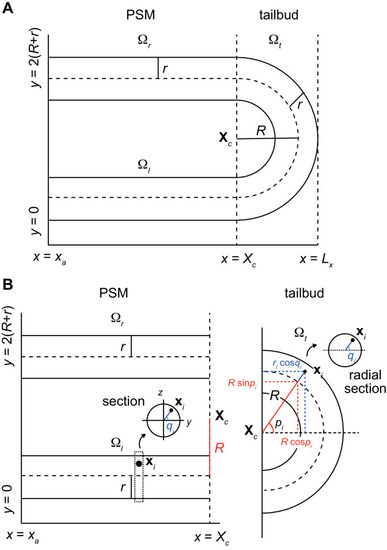
The z-axis is perpendicular to the paper. (B) Position of cell i can be expressed with a radial distance ri from the center of core curve of torus or that of tubes, and two angles pi and qi.

(A) Snapshots of a resynchronization simulation. Color scale as in Figure 2A, also in (D) and (F). The black dotted vertical line indicates the position of the anterior end of the PSM xa = 0. Tissue parameters are constant over time. See also Figure 3?video 1. (B-F) Analysis of local phase order and vortex transport in the simulation shown in (A). (B) Kymograph of local phase order parameter of the right PSM shown in (A). (C) Kymographs of phase vorticity for (left) clockwise and (right) counter clockwise rotations. The phase patterns within the black and yellow boxed space-time domains in (B) and (C) are shown in (D). (D) Snapshots of a phase vortex. The yellow arrows indicate the direction of rotation. (E) Local phase order parameters along the anterior-posterior axis of the PSM at different time points. (F) Time series of local phase order parameter at the anterior end of the right PSM xa. The horizontal broken line indicates the threshold Zc = 0.85 for determining normal and defective segments in simulations. The resultant stripe pattern is on top. In (A), (B) and (F), the blue and green triangles mark FRS and PLD, respectively. Red bracket in (F) highlights a segmental defect resulting from vortex in (D). Parameter values for simulations are listed in Supplementary file 1. (G), (H) Defect size distributions for (G) simulation (n = 800) and (H) embryonic experimental data (n = 134). Defect size indicates how many consecutive segment boundaries are defective in between FRS and PLD. In (G) and (H), the data for different washout timing shown in Figure 4 and Figure 1?figure supplement 1 were pooled to make the histograms. The defect size distribution for each washout timing is shown in Figure 3?figure supplement 3.

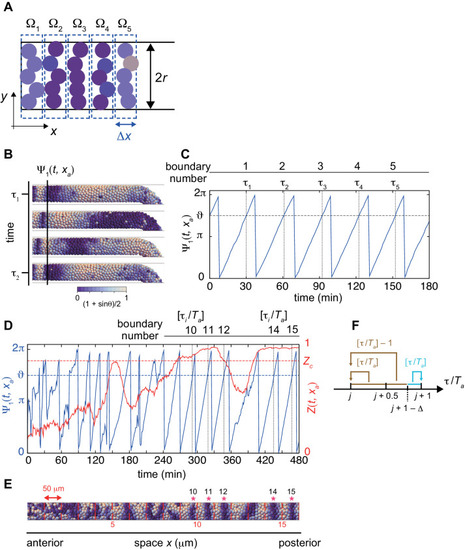
(A) Calculation of local phase order. Kuramoto phase order parameter Zm in each domain ?m (m = 1, 2,. . 5) are first calculated. The average over these domains is defined as a local phase order. Colored circles indicate cells. The width of the domain ?x is equal to the cell diameter dc, ?x=dc and 5?x is approximately one segment size. (B) Detection of a segment boundary position by the mean phase at the position xa. Scale bar as in Figure 2A, indicates the mapping of phase ?i to color: white is ?/2 and blue is 3?/2, also in (E). (C) Time series of the mean phase at the position xa. When the value of mean phase becomes ?, a segment boundary is considered to be formed. ?i indicates times at which segment boundaries are formed. In (B) and (C), a simulation was started from a synchronized initial condition for illustration. (D) Time series of the mean phase (blue) and local phase order (red) at the position xa. The red dotted line indicates the threshold for the local phase order to determine normal boundaries. ?i indicates time when the value of the mean phase surpasses ?. Ta is the period of oscillation at the position xa. (E) Formed segment boundaries. The asterisks indicate normal segment boundaries. The red vertical lines indicate expected segment boundary positions. (F) Assignment of segment boundary number. See Materials and methods for details.

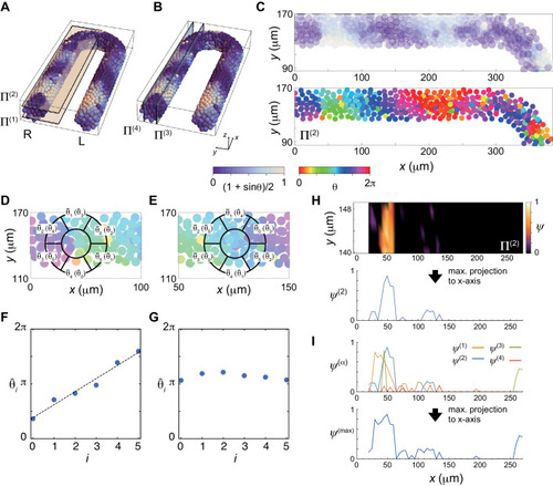
(A), (B) Planes ?(i) for vorticity calculation. Scale bar as in Fig. 2A, indicates the mapping of phase ?i to color: white is ?/2 and blue is 3?/2. (C) Phase distribution in ?(2) of the right PSM, (top) phase is color coded as in (A, B) and (bottom) color coded as indicated in the color bar. (D), (E) Average phase ?̄k of the subdomain Vk of a ring located at a lattice point. ??i is the permutation of ?̄k. A phase vortex is present in the region shown in (D), whereas there is no vortex in (E). (F) Linear increase of the values of ??i along the perimeter of the ring shown in (D). The black line indicates a linear fit to the data points. The vorticity is defined as (?̂5??̂0)/2?. (G) If there is no phase vortex as shown in (E), ??i does not increase linearly. (H) (top) Spatial distribution of the vorticity in ?(2). (bottom) The vorticity is projected to x-axis as ?(2). (I) Maximum projection of ?(i) obtained in each plain ?(i) to x-axis.

(A)-(E) Defect size distributions for different washout timing in embryonic experimental data. Washout at (A) t_wash-out = 9.5 hr post fertilization (hpf: 0 somite stage (ss); n = 28), (B) 11 hpf (3 ss; n = 22), (C) 12.5 hpf (6 ss; n = 28), 14 hpf (9 ss; n = 30) and 15.5 hpf (12 ss; n = 26). Defect size indicates how many consecutive segment boundaries are defective in between FRS and PLD. (F)-(G) Defect size distributions for different washout timing in simulation data. Washout at (F) t_wash-out = 0 ss, (G) 3 ss, (H) 6 ss, and (I) 9 ss. Simulation data for both left and right segments from 100 realizations in each washout timing are plotted. The model for the simulations includes the PSM shortening, change in cell advection pattern and increase in the coupling strength. The defect size was analyzed with the same simulation and experimental data shown in Figure 4 in the main text.

(A) Shapes of the speed of intrinsic mobility gradient v₀(x) in Equation (3) in the Materials and methods for different values of the maximum speed at the tailbud v_s. The origin of the horizontal axis is the anterior end of the PSM xa, x-=x-xa. (B) Time evolution of the mean squared difference of displacement vector (MSDD) for different values of v_s. The grey circles and squares indicate the MSDDs of two 17 somite-stage embryos quantified previously (Uriu et al., 2017, in the main text) as references. (C) Dependence of FRS (blue) and PLD (green) on v_s. The box-whisker plot indicates (0.05, 0.25, 0.75, 0.95) quantiles of FRS and PLD for 100 realizations of simulations. The white bars indicate median. The shaded interval of v_s is the range within which simulated MSDD is close to those from embryonic tissues shown in (B).

(A) PSMs with different lengths. Color scale as in Figure 2A. (B) Kymographs of vorticity for the different PSM lengths (left: 300 µm and right: 600 µm). Vorticity of the right PSM is shown. Trajectories of counter-clockwise vortices for PSM length L = 300 µm and L = 600 µm are presented. (C) Dependence of FRS (blue) and PLD (green) on the PSM length L. The box-whisker plot indicates (0.05, 0.25, 0.75, 0.95) quantiles of FRS and PLD for 100 realizations of simulations. The white bars indicate median.

(A) Advection speed vd (blue) as a function of normalized position, x-/L=x-xa/L. vp is the strain rate that is the magnitude of spatial derivative of advection speed (red) at the posterior part of the PSM (xq<x-/L). A smaller vp (top: vp=0.16) represents a lower strain rate at the posterior part than the anterior part of the PSM. A larger vp (bottom: vp=3) represents a larger strain rate in the posterior part of the PSM. (B) Kymographs of vorticity for (left) vp=0.16 and (right) vp=3. Vorticity across the right PSM is shown. Trajectories of counter-clockwise vortices are presented. (C) Dependence of FRS (blue) and PLD (green) on vp. The box-whisker plot indicates (0.05, 0.25, 0.75, 0.95) quantiles of FRS and PLD for 100 realizations of simulations. The white bars indicate median.

(A) Snap shots of the spatial phase patterns in the PSM with different values of r. Color scale as in Figure 2A. The black vertical lines indicate the anterior end of the PSM x_a. (B) Dependence of FRS (blue) and PLD (green) on r. The box-whisker plot indicates (0.05, 0.25, 0.75, 0.95) quantiles of FRS and PLD for 100 realizations of simulations. The white bars indicate median.

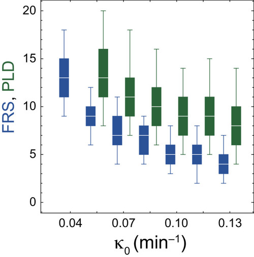
The dependences of FRS (blue) and PLD (green) on κ0 are shown. The box-whisker plot indicates (0.05, 0.25, 0.75, 0.95) quantiles of FRS and PLD for 100 realizations of simulations. The white bars indicate median. Note that PLD for κ0=0.04 was not well-defined because a low value of coupling strength could not maintain a higher level of synchrony Z(t) > Z_c in the presence of cell addition with random phase values. Even when a simulation was started from the completely synchronized state, Z(t) sometimes became lower than Z_c. Therefore, the result of PLD for a such small value of κ0 is not plotted in the figure.

(A)-(C) Snapshots of spatial phase patterns in desynchronization simulations with (A) the phase noise intensity Dθ=0 min^–1, (B) Dθ=0.0013 min^–1 and (C) Dθ=0.0026 min^–1. In these simulations, coupling strength was set to zero κ=0 in Equation (10). Color scale as in Figure 2A. The black vertical lines indicate the position of the anterior end of the PSM xa. (D) Time evolution of local phase order parameter Z at xa for different values of Dθ in the desynchronization simulations with κ=0. Marks and error bars indicate averages and standard deviations of Z, respectively, for 10 realizations of simulations. (E) Dependence of FRS (blue) and PLD (green) on the phase noise intensity Dθ in resynchronization simulations in a constant tissue with κ0=0.07. The box-whisker plot indicates (0.05, 0.25, 0.75, 0.95) quantiles of FRS and PLD for 100 realizations of simulations. The white bars indicate median. In all panels, the PSM length and advection pattern were constant over time.

(A) Frequency profile U(x) for different values of k in Equation (11) in the Materials and methods. x-=x-xa where xa is the position of the anterior end of the PSM. (B) Snap shots of spatial phase patterns with different values of k. Simulations were started from synchronized initial conditions for illustration. Color scale as in Fig. 2A, xa is indicated by the black vertical lines. (C) Dependence of FRS (blue) and PLD (green) on k in resynchronization simulations from random initial conditions. The box-whisker plot indicates (0.05, 0.25, 0.75, 0.95) quantiles of FRS and PLD for 100 realizations of simulations. The white bars indicate median.

(A) Snap shots of the spatial phase patterns in the PSM with different values of R. Color scale as in Figure 2A. The black vertical lines indicate the anterior end of the PSM x_a. Simulations were started from synchronized initial conditions for illustration. (B) Dependence of FRS (blue) and PLD (green) on R in resynchronization simulations. The box-whisker plot indicates (0.05, 0.25, 0.75, 0.95) quantiles of FRS and PLD for 100 realizations of simulations. The white bars indicate median.

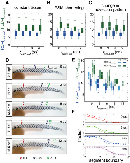
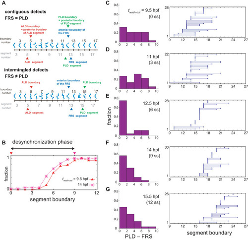
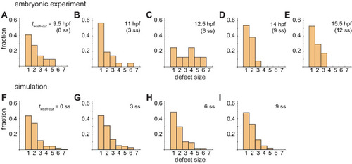
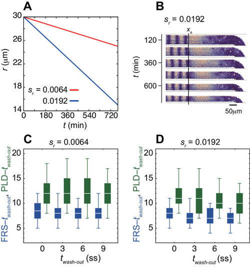
(A-C) Dependence of times to FRS and PLD on DAPT washout time for different conditions in simulations. (A) Constant tissue where all the tissue parameters remain unchanged during a simulation. (B) PSM length becomes shorter with time. All the other parameters are constant. See also Figure 4?video 1. (C) Cell advection pattern changes at 9 somite stage (ss). Before 9 ss, the strain rate is larger in the anterior than posterior PSM. After 9 ss, the strain rate becomes larger in the posterior PSM. See also Figure 4?video 2. All the other parameters are constant. The box-whisker plots indicate 5, 25, 75, and 95 percentiles. The white bars mark the median. In (B) and (C), the gray dotted lines mark the medians of FRS and PLD in the constant tissue shown in (A). (D) Whole-mount in situ hybridization for the myotome segment boundary marker gene xirp2a in ~36 hr post-fertilization (hpf) embryos. DAPT washout time is 9.5 hpf (0 ss; n = 28), 11 hpf (3 ss; n = 22), 12.5 hpf (6 ss; n = 28), 14 hpf (9 ss; n = 30), and 15.5 hpf (12 ss; n = 26) from top to bottom. Red, blue and green triangles indicate the ALD, FRS, and PLD, respectively. (E) Dependence of times to FRS and PLD on DAPT washout time. Light blue and green box-whisker plots indicate 5, 25, 75, and 95 percentiles for embryonic experimental data (exp.). Dark blue and green box-whisker plots indicate those for simulation data (sim.). The white bars mark the median. The PSM shortening, change in cell advection pattern and increase in the coupling strength are combined in the model, see also Figure 4?videos 3 and 4. The lack of information about the formation of final segments in embryos precludes simulations for the latest washout (12 ss), see the text. (F) Spatial distribution of segment boundary defects. Symbols indicate embryonic experimental data and lines indicate simulation data. Grey dashed vertical line across panels is a guide to the eye. In (A-C), (E), results of 100 realizations of simulations with each washout timing are plotted. Parameter values for numerical simulations are listed in Supplementary files 1 and 2. Source data for (D-F) is available in Figure 1?source data 1.

(A) Time evolution of the PSM length at different speed of PSM shortening u_a. (B) Kymographs of vorticity for washout time at t_wash-out = 0 min (0 somite-stage, ss: left) and 270 min (9 ss: right). The black triangles indicate timing of washout. The wshite solid lines indicate the position of the anterior end of the PSM x_a. Vorticity across the right PSM is shown. Trajectories of counter-clockwise vortices for t_wash-out = 0 min and those of clockwise vortices for t_wash-out = 270 min are presented. (C) Dependence of time to PLD, PLD – t_wash-out, on u_a for different washout timing t_wash-out. Medians for 100 realizations of simulations are plotted. (D-F) Dependences of time to FRS, FRS – t_wash-out (blue) and time to PLD, PLD – t_wash-out (green) on t_wash-out for different values of u_a. (D) u_a = 0.1, (E) 0.4 and (F) 0.66. The box-whisker plot indicates (0.05, 0.25, 0.75, 0.95) quantiles of times to FRS and PLD for 100 realizations of simulations. The white bars indicate median.

(A) Change in advection pattern at t = t_g. The blue and red lines indicate the advection speed v_d and strain rate, respectively. x-=x-xa where xa is the position of the anterior end of the PSM. (B), (C) Kymographs of vorticity for washout at (B) t_wash-out = 0 min (0 somite stage; ss) and (C) 270 min (9 ss). White dotted lines indicate t_g at which the advection pattern changes (t_g = 9 ss). Vorticity across the right PSM is shown. Trajectories of clockwise vortices for t_wash-out = 0 min and those of counter-clockwise vortices for t_wash-out = 270 min are presented. (D-G) Dependence of times to FRS (blue) and PLD (green) on washout time t_wash-out with change in advection pattern at (D) t_g = 6 ss, (E) 9 ss, (F) 12 ss, and (G) 15 ss. The gray dotted lines indicate times to FRS and PLD for the constant tissue shown in Figure 4A in the main text. The box-whisker plot indicates (0.05, 0.25, 0.75, 0.95) quantiles of times to FRS and PLD for 100 realizations of simulations. The white bars indicate median.

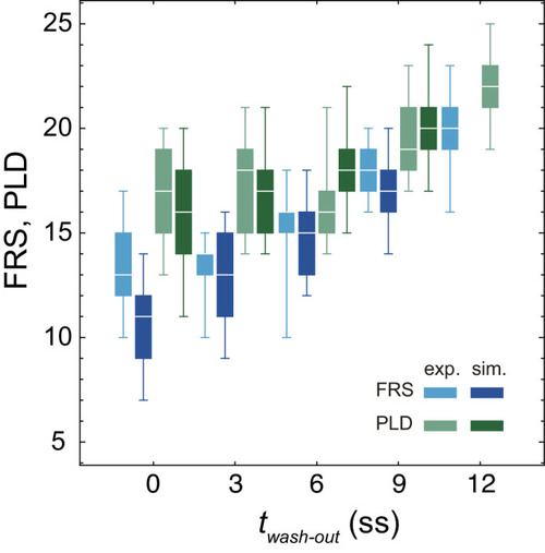
Experimental FRS (light blue) and PLD (light green) for zebrafish embryos are plotted together with FRS and PLD (darker colors) obtained by 100 realizations of numerical simulations. The physical model for the simulations included PSM shortening, changes in advection pattern and coupling strength. The box-whisker plot indicates (0.05, 0.25, 0.75, 0.95) quantiles of FRS and PLD. The white bars indicate median. Due to the lack of the information about the formation of final segments, we did not perform simulations for the latest washout t_wash-out = 12 somite-stage (ss), see the main text. exp.: experiment. sim.: simulation.

(A) PSM radius r as a linear function of time. s_r represents the absolute value of slope of a linear line. (B) Snapshots of spatial phase patterns of a simulation with decreasing PSM radius. The simulation was started from a synchronized initial condition for illustration. Color scale as in Figure 2A. The black vertical line indicates the position of the anterior end of the PSM x_a. (C), (D) Dependence of times to FRS (blue) and PLD (green) on t_wash-out with (C) s_r = 0.0064 μm min^–1 (red line in A) and (D) s_r = 0.0192 μm min^–1 (blue line in A). Only the PSM radius changed over time, whereas all the other parameters were kept constant. Simulations were started from random initial conditions. The box-whisker plot indicates (0.05, 0.25, 0.75, 0.95) quantiles of times to FRS and PLD for 100 realizations of simulations. The white bars indicate median. ss: somite stage.

(A) Time series of the coupling strength κ with different DAPT washout time in the physical model. Black dashed lines indicate the increase of coupling strength over developmental stages in the absence of DAPT treatment. Red solid lines indicate coupling strength before and after DAPT washout. For simplicity, we assume that cells restore coupling to its original value immediately after washout as represented by the vertical red lines. (B) Dependence of times to FRS (blue) and PLD (green) on DAPT washout time in simulations. The box-whisker plot indicates (0.05, 0.25, 0.75, 0.95) quantiles of times to FRS and PLD for 100 realizations of simulations. The white bars indicate median. The effect of increasing coupling strength shown in (A) was examined with the constant PSM length and advection pattern. ss: somite stage.

(A), (B) Kymographs of vorticity for (A) t_wash-out = 0 somite stage (ss; 0 min) and (B) t_wash-out = 9 ss (270 min). The white horizontal dotted lines indicate time t_g at which advection pattern changes, t_g = 240 min. The solid white lines indicate the position of the anterior end of the PSM x_a. Vorticity across the right PSM is shown. Trajectories of clockwise vortices are presented.

(A) Spatial distribution of defective segments in left (red lines: p_l) and right (blue lines: p_r) sides of embryos. (B) Spatial probability distribution of ALD qa (red lines), FRS qf (blue lines) and PLD qp (green lines) for different DAPT washout time calculated from the spatial distribution of defective segments px. Symbols indicate direct measurement of qa (triangles), qf (squares), and qp (circles). See Supporting Information for calculation. (C) ALD, FRS and PLD as a function of DAPT washout timing. Symbols indicate results of direct measurement of these quantities. Lines indicate results of probability calculations described in Supporting Information. ss: somite stage.

(A) Spatial probability distribution of single defects p_s (red lines) and double defects p_d (blue lines) for different DAPT washout time. p_s and p_d were calculated from the experimental spatial distributions of defective segments. Filled circles indicate direct measurement of p_s (red) and p_d (blue). (B) Comparison of p_s (red) and p_d (blue) between simulations (dotted lines) and experiment (solid lines). (C) Dependence of fraction of single defects F_s on DAPT washout timing. Circles indicate F_s obtained by direct measurement. Error bars indicate the standard deviation. The line indicates F_s calculated from the spatial distribution of defective segments. See Supporting Information for the calculation. F_s was computed using entire segment range. (D) Comparison of F_s obtained by the physical model (lines) with that in experiment (circles). The solid and dotted lines indicate mean and standard deviations of simulation data, respectively. F_s was measured from segment 9 for the comparison between simulations and experiment.