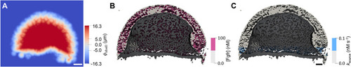
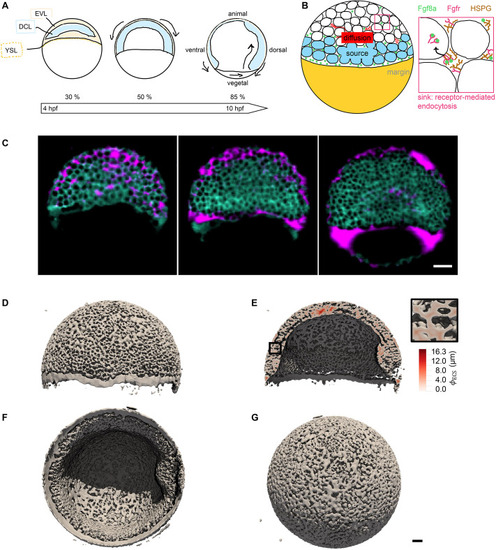
The extracellular space resembles an anisotropic porous medium during zebrafish epiboly. (A) Illustration of zebrafish epiboly. Representative stages at around 40%, 50% and 85% epiboly with deep-cell layer (DCL, blue), enveloping layer (EVL, yellow) and yolk syncytial layer (YSL, yellow dots). Starting at around 4 hpf (40% epiboly), the yolk moves toward the animal pole, and the blastoderm, which is composed of EVL, DCL and YSL, starts spreading over the yolk. Toward the end of epiboly, the blastoderm almost completely engulfs the yolk, and asymmetry along the dorsal-ventral axis emerges. (B) Scheme of Fgf8a gradient formation during zebrafish epiboly. Secreted by source cells at the blastoderm margin (blue), Fgf8a diffuses along tortuous paths through the ECS, further hindered by HSPG binding. The complex formation of Fgf8a, HSPG and Fgf receptors initiates internalization and endocytosis of Fgf8a into target cells acting as sinks (pink-framed box). (C) Light-sheet microscopy images of zebrafish epiboly. From left to right: exemplary optical sections from a Tg(bactin:hRas-EGFP) embryo at late blastula, early gastrula and mid-gastrula stages, respectively, following image acquisition using a light-sheet fluorescence microscope and multi-view reconstruction (see the section ‘Acquisition of light-sheet microscopy time-lapse video’). hRas-EGFP labels the cell membranes (green). ECS is marked by TMR-dextran injection (magenta). Unidirectional views and single optical sections are shown for simplicity. For all 25 timepoints, see Movie 1. (D-G) Visualization of the sparse-grid discretization of the ECS at ≈60% epiboly. (D) Side view oriented as in B and C. (E) Cross-sectional view with φ_ECS values in increasing distance to the ECS surface shown in shades of red (color bar). (F) Cross-sectional views from the vegetal pole. (G) View from the animal pole. Scale bars: 50 μm.

A SDD+HSPG mechanism is sufficient to explain the formation of the Fgf8a gradient in realistic ECS geometries. All Fgf8a concentrations in the simulation were initially set to zero throughout the embryo. (A) Evolution of the emerging AV gradient profile of (Fgf8a - total) over time (colored bar). The gradient reaches a steady state at ≈30 min. (B) The Fgf8a-free/Fgf8a:HSPG^ECS ratio remains almost constant (92.6%/7.4%) and close to the experimentally measured values (93%/7%) throughout the 60 min of simulated time. (C) Visualization of the simulated Fgf8a-total concentrations in the ECS geometries at 40%, 60% and 75% epiboly. (D) Simulated (lines) and experimentally measured (symbols) AV profiles at different stages (see key). Experimental profiles were only available at 60% and 75% epiboly, and show the mean over N = 15 embryos. Simulated profiles are computed at . Scale bar: 50 μm.

Sensitivity of the simulated steady-state Fgf8a gradients to variations in the model parameters and in vivo gradient sensitivity to HepI injection. (A,B) The normalized simulated gradient shows remarkable robustness against changes in source (A) and sink rates (B) over four orders of magnitude (see key). (C,D) Changes in the effective diffusivity, by changing either the molecular diffusion coefficient of Fgf8a (C) or HSPG concentrations (D), strongly affect the gradient. The higher the HSPG binding and the smaller the diffusion coefficient, the steeper and shorter the gradient. The baseline gradient (see the section ‘A SDD+HSPG-binding mechanism is sufficient to generate de novo Fgf8a gradients’) is shown as a solid black line in all panels. All profiles are normalized by their respective maximum xz-plane-averaged concentration. Profiles are shown at . (E) FCS count rates of Fgf8a without (black squares) and with (orange circles) HepI injection. HepI cleaves off the HS side-chain of HSPGs. The Fgf8a gradient of HepI-injected embryos is shallower. Reproduced, with permission, from Harish et al. (2023). N=20 embryos for control, N=13 for HepI; data are mean±s.d. (F) The gradient decay lengths λ scale linearly with the square root of the molecular diffusion coefficient of the morphogen, as expected for gradients forming by an SDD mechanism (Kicheva et al., 2012; Hidalgo et al., 2019 preprint). The linear fits show the least-squares solutions obtained using numpy.linalg.lstsq (Harris et al., 2020). The key provides the fitted proportionality coefficients and the respective goodness of fit R².

ECS geometry controls Fgf8a gradient steepness and range. To test how ECS tortuosity influences Fgf8a gradients, we simulated de novo gradient formation for different ECS geometries. (A) Clipped visualizations of the baseline ECS geometry (center) and two perturbed versions (left and right) with simulated Fgf8a concentrations overlaid in green, scaled to (see color intensity bar). The ECS tube thickness is perturbed by changing the boundary location along φ_ECS: shifting down by one grid spacing h=0.915 μm (2 pixels), i.e. φ_ECS=− 0.915 μm, to obtain thicker tubes; and increasing by 3h, i.e., φ_ECS=2.745 μm to obtain thinner tubes. (B) Higher magnification images of the areas outlined in A. (C) Absolute AV concentration profiles at . Colors correspond to different geometries (see key). Compared to the baseline geometry (solid black line), decreasing ECS tube sizes limits Fgf8a propagation lengths and leads to a steeper gradient with a higher peak (gray lines), whereas increasing the ECS tube size leads to a flatter gradient (violet line). (D) The same profiles normalized to their respective maximum concentration values. The in vivo profile at 60% epiboly (symbol) is more similar to the simulated profile for thinner tubes of φ_ECS=1.830 μm, the average decay length of which, , is close to the in vivo decay length λ. (E) Linear scaling of λ^I and λ^II with respect to . The linear fit is the least-squares solution obtained using numpy.linalg.lstsq (Harris et al., 2020). The key provides the fitted proportionality coefficients and their goodness of fit R². Scale bars: 100 μm (A); 10 μm (B).

Steps for modeling ECS geometries from light-sheet microscopy volumes. Volumes are visualized for an exemplary time point (12 out of 25, ≈60% epiboly) and z-slice (plane 480 from the epiblast in the direction of hypoblast and the yolk, i.e. the mid-plane formed by the AV/DV axes). (A) TMR-dextran channel of the light-sheet data after 3D multi-view fusion; fluorescence marks the ECS. (B) Segmentation mask of the ECS (white) with a yellow dashed line showing the margin plane and pink circles highlighting specks of noise and small unconnected islands that were subsequently removed. (C) Binary indicator function of the ECS after mask denoising and horizontal alignment of the margin plane (yellow dashed line). (D) Re-distanced signed-distance function, φ_ECS, of the level-set representation of the ECS surface. (E) Sparse block grid storing only points in the ECS. Scale bars: 50 μm.

Spatially varying sources and sinks in the 3D model at an exemplary time point at ≈60% epiboly. (A) Signed-distance function (SDF) of the embryo shell boundary, φ_shell, for an exemplary z-slice. Combining φ_shell (representing YSL and EVL boundaries) with φ_ECS enables the restriction of sources and sinks to the deep-cell surfaces. (B,C) A clipped model of the ECS showing that Fgf receptors (B, pink) are restricted to the deep cell boundaries, i.e. not the EVL or YSL. The sources (C, blue) are restricted to ≈5 rows of deep cells above the margin of the blastoderm. Receptor concentrations are given in units of nM; k_source is given in nM/s. Scale bars: 50 μm.

Initialization of the total Fgf8a concentration with the experimental fluorescence intensity profile at ≈60% epiboly. (A) The fluorescence intensity profile (right) is extracted from sum-intensity z-projected confocal images (left). Values are intensity averages across a 100 μm wide region (neural plate). Reproduced, with permission, from Harish et al. (2023). The embryo is oriented as in Fig. 1B (ventral left, dorsal right, animal pole top, vegetal pole bottom). N=15 embryos. Data are represented as mean±s.d. (B) The concentration field in the simulation (left) was obtained by linearly interpolating between the discrete margin distances of the experimental profile and uniformly distributing the mass in each xz-plane. We converted normalized intensity values to concentrations by scaling with the maximum concentration measured by FCS. For comparison with experiments, we computed 1D profiles (right) along the AV axis by averaging the total Fgf8a concentration in each xz-plane. The model has the same orientation as the embryo in A. Scale bars: 50 μm.

Simulated Fgf8a gradient using optimized parameters with experimental profile as initial condition. For parameters, see Table 2. (A) Normalized AV concentration profiles of Fgf8a-total at different simulated times (see color intensity bar). All profiles are normalized by their respective maximum xz-plane-averaged concentration. The experimental profile used as the initial condition is shown in dark purple (time 0). Simulated profiles reach a steady state within 12 min. (B) Normalized total mass of two Fgf8a fractions, Fgf8a:HSPG^ECS and Fgf8a-free, along with their sum (Fgf8a-total). This set of parameters maintains a constant total Fgf8a mass and preserves the in vivo Fgf8a/Fgf8a:HSPG^ECS ratio of 93%/7%.

Initial condition of simulated FRAP experiment in the ECS geometry and the shell geometry. (A) ECS geometry and (B) shell geometry. The lower half of the ECS is uniformly initialized with [Fgf8a]=0.001 (arbitrary unit), and the upper half (above 500 μm above the margin) with [Fgf8a]=0. To estimate the diffusive hindrance of ECS tortuosity alone, we simulate diffusion without reactions, measuring the total mass recovery in the bleached half. Fitting the recovery curve of the shell geometry to the curve of the ECS geometry, we find the ratio between the local and effective diffusion coefficient, i.e. the tortuosity factor τ_d=2.5. Scale bar: 50 μm.

Porous-media characteristics of ECS can be partly upscaled in a shell geometry. (A-C) Clipped simulation visualization of (A) the source in a 70 μM DCL band at the margin, (B) the uniformly distributed sink ([Fgfr]) in the DCL, and (C) the Fgf8a gradient at (concentration color bar) using the parameters from Table 2. (D) Modeling the ECS geometry as a spherical shell without HSPG leads to a longer, flatter gradient (orange dashed line) compared to the baseline of the pore-scale model (black line). Gradient steepness and range are partly recovered by upscaling HSPG binding by uniformly distributed HSPG^ECS and HSPG^cellSurf, and they are fully recovered when further upscaling the tortuosity by an effective diffusion coefficient using τ_d (as defined in the section ‘Determining the ECS diffusive tortuosity to quantify geometric hindrance’). However, this does not apply to local geometry effects such as the zonation near the source, as found in the in vivo profile (indicated by cyan crosses) and reproduced by the pore-scale model. AV profiles are reported at . Scale bar: 50 μm.

Asymmetry in ECS geometry could explain Fgf8a DV gradient. (A) The Fgf8-EGFP gradient in the ECS at midgastrula stage (≈75% epiboly). The normalized fluorescence intensity profile in the ventral-to-dorsal direction (right) was extracted from sum-intensity z-projected confocal images (left). Values are intensity averages across a region at the marginal blastomere (dotted yellow lines); N=10 embryos. Data are mean±s.d. The embryo is oriented as in Fig. 1A (ventral left, dorsal right, animal pole top, vegetal pole bottom; see gray schematic). Reproduced, with permission, from Harish et al. (2023). (B) Simulated de novo Fgf8a gradient and DV concentration profiles at ≈75% epiboly. The concentration profiles in the ventral-to-dorsal direction (right) were computed by averaging concentration values over yz-planes within the marginal region (dashed yellow lines). The model has the same orientation as the embryo in A. Color represents concentrations in nM (see intensity bar on the left) and simulated time of gradient formation (see color intensity bar on the right). Scale bars: 50 μm. (C) Simulated normalized de novo Fgf8a DV concentration profiles at different stages of epiboly (see key). A gradient similar to the one observed in vivo (A) emerges at ≈75% epiboly. The computationally predicted profiles are flat in geometries of 40% and 60% epiboly (gray and cyan lines, respectively). All profiles are computed at . (D) ECS porosity (plus symbols) along the DV axis at different stages of epiboly (see key). At 75% epiboly, the ψ_ECS profile shows a gradient with porosity values approximately halving from ≈0.4 at the ventral to ≈0.2 at the dorsal side. The hypothesis that this could explain the Fgf8a DV gradient is contradicted by the similar ψ_ECS profile at 60% epiboly, which is when the Fgf8a DV profile is flat.

Using porosity profiles along the AV axis for upscaling in a 1D model. (A) Comparison of the ECS porosity (plus symbols, right y-axis) and [Fgf8a-total] profiles (lines, left y-axis) along the AV axis at different stages of epiboly (see key). In the first 100 μm from the margin, where the profile has a kink, ψ_ECS approximately doubles. All profiles are computed at . (B) AV profiles of the ECS porosity, ψ_ECS (black symbols); the source, ψ_source (solid light-blue line); and the sink, ψ_[Fgfr] (dashed pink line). All profiles are computed according to Eqn 15 by dividing the volume of the respective phase of interest by the total volume of the embedding spherical shell. (C) Upscaling SDD in porous ECS geometries. To disentangle the role of porous ECS heterogeneity in source, diffusion and sink on the formation of the AV gradient kink, we accounted for the AV profiles of ψ_ECS, ψ_source and ψ_[Fgfr] by linearly scaling (1) D_Fgf8a and with ψ_ECS (light-green line) and (2) f_source with ψ_source (light-blue line), and by (3) combining (1) and (2) (dark-green line), and (4) combining (3) with scaling [Fgfr] with ψ_[Fgfr] (pink line). The kink at the source is partly recovered when upscaling D_Fgf8a and f_source (case 3, dark-green line). All profiles are normalized by their maximum concentration and shown at .

Sensitivity of a 1D model to variations in the model parameters. (A,B,G) Similar to the 3D model, the normalized simulated gradient shows robustness against changes in rates of source (A) and sink [i.e. k_internalize (B) and k_complex (G)] (see key). (C,D) Changes in the effective diffusivity, by changing either the molecular diffusion coefficient of Fgf8a (C) or HSPG concentrations (D), strongly affect the gradient. The stronger the HSPG binding and the smaller the diffusion coefficient, the steeper and shorter the gradient. (E,F) Higher HSPG affinities (E) lead to shorter and steeper gradients with higher amplitude at the source (see absolute concentrations in Fig. S7E), whereas reducing HSPG unbinding rates (F) does not affect the gradient shape. (H) Compared to the baseline, decreasing [Fgfr] leads to flatter gradients, whereas increasing [Fgfr] has almost no effect on the gradient. This could be because of the HSPG binding that precedes Fgfr binding in our model, which could be the limiting step. For the baseline gradients, shown as a solid black line in all panels, the same parameters were used as in the 3D model (Table 2). All profiles are normalized by their respective maximum concentration. Profiles are shown at , which for complex internalization rates 100 times smaller and all HSPG binding rates larger than the baseline is before the gradient has reached steady state. This agrees with previous analytical solutions showing that steady state is reached slower for higher non-receptor binding (Lander et al., 2007) and smaller degradation rates (Berezhkovskii et al., 2010; Gordon et al., 2013).

Fitting exponential decay to in vivo and simulated gradients. (A) Exponential decay fit to in vivo 1D and 3D model gradients (dashed lines, see key). The in vivo gradient was best fitted in the range 40 μm≤d≤161 μm. For the 1D model, the source region was excluded from the fit, i.e. d≥70 μm. The gradient of the 3D model was best fitted by a mixture of two exponential functions: the first for 35 μm≤d≤125 μm and the second for d>125 μm. (B) Fit to image-based 3D simulation gradients for different Fgf8a diffusion coefficients. (C) Exponential decay fit to 1D model simulation gradients for different Fgf8a diffusion coefficients. (D) Exponential fit to gradients of different ECS tube thicknesses. All curves were fitted using the non-linear least squares function curve_fit from the scipy.optimize library (Virtanen et al., 2020). The key provides the fitted proportionality coefficients and their goodness of fit R².