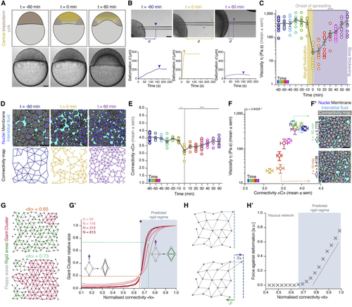
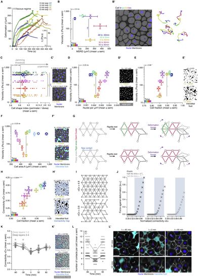
Blastoderm cell connectivity as a potential control parameter of a tissue rigidity percolation transition

(A) Schematic representations (top) and bright-field single-plane images (bottom) of an exemplary embryo before (t = −60 min), at the onset (t = 0 min), and after blastoderm spreading (t = 60 min). The yellow-shaded region represents the central blastoderm.

(B) Exemplary bright-field images of creep and recovery aspiration experiments in the central blastoderm at the stages described in (A) (top) and corresponding deformation (d) plots showing the distance covered by the tissue in the pipette under constant pressure as a function of time (bottom). Arrowheads indicate the deformation at pressure release.

(C) Dot plot of individual viscosity values of the central blastoderm obtained from the aspiration experiments shown in (B) overlaid with a line plot of the mean ± SEM as a function of time (color coded for 10 min intervals) (n = 129 embryos, N = 12 embryo batches). Gray dashed line indicates the onset of blastoderm spreading during the fluidization (yellow shade)/thickening (purple shade) process.

(D) Exemplary 2D confocal sections at the 1^st–2^nd deep-cell layer of the blastoderm (top) and their connectivity maps (bottom) at the stages described in (A). Interstitial fluid is marked by dextran, nuclei by H2B-GFP, and membranes by membrane-red fluorescent protein (RFP).

(E) Dot plot of individual connectivity <C> values (number of contacts/cell) obtained from central blastoderm confocal sections overlaid with a line plot of the mean ± SEM as a function of time (color coded) (n = 11 embryos for time points −60, −30, 0, 30, and 60 min; n = 6 embryos for all other time points; N = 11 embryo batches). Gray dashed line indicates the onset of blastoderm spreading.

(F) Plot of the central blastoderm viscosity values (mean ± SEM) as a function of connectivity <C> (mean ± SEM) over time (color coded as in E; for viscosity n = 129 embryos, N = 12 embryo batches; for connectivity n = 103 blastoderms, N = 11 embryo batches).

(F’) Two exemplary blastoderm confocal sections (marked as in D) with overlaid connectivity maps displaying slightly different connectivity, but by an order of magnitude different viscosity values.

(G) Exemplary simulated networks with normalized connectivity <k> values above (green line in G’) and below (orange line in G’) the critical point (asterisk in G’) of the rigidity percolation transition. Floppy areas are illustrated in gray, rigid areas in green, and the giant cluster (GC) in red.

(G’) Plot of the fraction of the network occupied by the GC as a function of normalized connectivity <k> in simulated random 2D triangular lattices of different sizes (N, number of nodes). The gray-shaded area indicates the network rigid regime above the critical connectivity point (k_c, black asterisk). The schematics illustrate how, under the same deformation force (purple arrow), a floppy (left, costing zero energy) or rigid (right, costing non-zero energy due to its central bond) cluster of nodes would deform.

(H) Schematic diagram of the force response (F, green arrow) for set deformation (δx, blue arrow) induced by a small displacement of the edge layer of viscous 2D networks.

(H’) Plot of the force response illustrated in (H) for viscous 2D networks of size N ∼ 250 nodes, as a function of normalized connectivity <k>. Bond half-life time τ is 2Te, where Te is the number of simulation time steps. The gray-shaded area indicates the rigid regime above the k_c, for which viscosity grows linearly as a distance from the critical point.

Kruskal-Wallis test (C and E), ρ Spearman correlation test (F). Scale bars: 100 μm in (A) and (B) and 50 μm in (D) and (F’).

See also Figure S1 and Video S1.

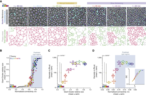
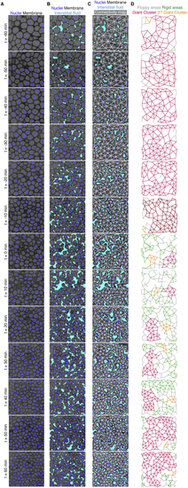
A tissue rigidity percolation transition describes the temporal blastoderm viscosity profile

(A) Exemplary 2D confocal sections at the 1^st–2^nd deep-cell layer of the central blastoderm with overlaid connectivity maps (top) and their rigidity profile (bottom) at consecutive time points during the fluidization/thickening process (color coded). Interstitial fluid is marked by dextran, nuclei by H2B-GFP, and membranes by membrane-RFP. Floppy areas are illustrated in gray, rigid areas in green, and the rigid GC in red. Shaded yellow and purple areas indicate the time period of tissue fluidization and thickening, respectively.

(B) Plot of the fraction of the network occupied by the GC (mean ± 95% confidence interval [CI]) as a function of normalized connectivity <k> in simulated random networks of the same size as the average size of experimental networks (black). Overlaid dot plot of the measured GC sizes as a function of the normalized connectivity <k> for experimental networks of the central blastoderm at different time points during the fluidization/thickening process (color coded for 10 min intervals) (n = 103 experimental networks, N = 11 embryo batches), agreeing with the theoretical expectation.

(C) Plot of tissue viscosity (mean ± SEM) as a function of the GC relative size (mean ± SEM) for experimental networks of the central blastoderm at different time points during the fluidization/thickening process (color coded as in B) (for viscosity n = 129 embryos, N = 12 embryo batches; for GC n = 103 blastoderms, N = 11 embryo batches). Statistical tests were performed in comparison to t = 0 min.

(D) Plot of tissue viscosity (mean ± SEM) as a function of normalized connectivity <k> (mean ± SEM) for the samples described in (C) (for viscosity n = 129 embryos, N = 12 embryo batches; for normalized connectivity <k> n = 103 blastoderms, N = 11 embryo batches). Statistical tests were performed in comparison to t = 0 min. The integrated plot illustrates the time trajectory (color coded) of the central blastoderm material phase state (relative size of GC) as a function of its connectivity (k_c).

The gray-shaded region in (B) and (D) indicates the rigid regime above the k_c.

Kruskal-Wallis test (C and D), ρ Spearman correlation test (C and D). Scale bars: 50 μm in (A).

See also Figure S2, Table S1, and Video S2.

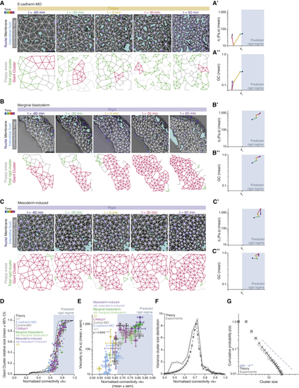
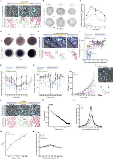
The blastoderm connectivity profile identifies key hallmarks of criticality during its rigidity percolation PT

(A–C) Exemplary 2D confocal sections at the 1^st–2^nd deep-cell layer of the central blastoderm of an e-cadherin-morpholino (MO)-injected embryo (A), of the marginal blastoderm of a WT embryo (B), and of the central blastoderm of a mesoderm-induced embryo (C) with overlaid connectivity maps (top) and their rigidity characteristics (bottom) during the fluidization/thickening process (color coded for 30 min intervals). Interstitial fluid is marked by dextran, nuclei by H2B-GFP, and membranes by membrane-RFP. Floppy areas are illustrated in gray, rigid areas in green, and the GC in red. Yellow- and purple-shaded areas indicate fluidized and rigid blastoderms, respectively.

(A’, B’, and C’) Plots of the time trajectory (color coded) of blastoderm viscosity (mean) as a function of its normalized connectivity <k> for e-cadherin-MO central blastoderm (A’; for viscosity n = 94, N = 6; for connectivity n = 54, N = 6), WT marginal blastoderm (B’; for viscosity n = 115, N = 9; for connectivity n = 15, N = 3), and mesoderm-induced central blastoderm (C’; for viscosity n = 42, N = 6; for connectivity n = 15, N = 3).

(A’’, B’’, and C’’) Plots of the time trajectory (color coded) of the GC relative size as a function of its normalized connectivity <k> for the samples described in (A’), (B’), and (C’).

(D) Plot of the fraction of the network occupied by the GC (mean ± 95% CI) as a function of normalized connectivity <k> in simulated random networks of the same size as the average size of WT experimental networks (black). Overlaid dot plot of the measured GC size as a function of the normalized network connectivity <k> of the central blastoderm in WT (n = 103, N = 11), e-cadherin-MO (n = 54, N = 6), control-MO (n = 15, N = 3), CAMypt1 (n = 89, N = 13), slb/wnt11f2 mutant (n = 10, N = 2), and mesoderm-induced WT (n = 15, N = 3) embryos and of the marginal blastoderm in WT (n = 15, N = 3) and slb/wnt11f2 mutant (n = 15, N = 3) embryos. n, number of networks; N, number of embryos.

(E) Plot of central blastoderm tissue viscosity (mean ± SEM) as a function of normalized connectivity <k> (mean ± SEM) for the experimental networks described in (D) (for viscosity: central blastoderm of WT n = 129, N = 11; e-cadherin-MO n = 94, N = 6; control-MO n = 71, N = 6; CAMypt1 n = 66, N = 7; slb/wnt11f2 mutant n = 54, N = 4; mesoderm-induced WT n = 42, N = 6; mesoderm-induced slb/wnt11f2 mutant n = 13, N = 3 embryos; marginal blastoderms of WT n = 115, N = 9; slb/wnt11f2 mutant n = 44, N = 5 embryos; for connectivity: samples described in D).

(F) Plot of the variance (Var) of the distribution of rigid cluster sizes p(s) other than the GC, as a function of their normalized connectivity <k>, in simulated networks of the same size as the average size of experimental networks (black) and in the experimental networks described in (D) (gray) (except marginal networks), showing divergence at the critical point, with good theory-experiment agreement.

(G) Plot of the cumulative distribution of rigid cluster sizes p(s) other than the GC near the critical point. The numerical experiment shows the scaling behavior of cluster size distribution p(s) for networks of arbitrary large size (∼1,200 nodes). The overlaid plot shows the cluster size distribution near criticality for real networks, showing excellent agreement with predictions. The dashed line shows a power-law p(s) ∼ s^−2.5.

The gray-shaded regions at the plots indicate the rigid regime above the theoretical k_c.

ρ Spearman correlation test (E). Scale bars: 50 μm in (A)–(C).

See also Figure S3 and Table S1.

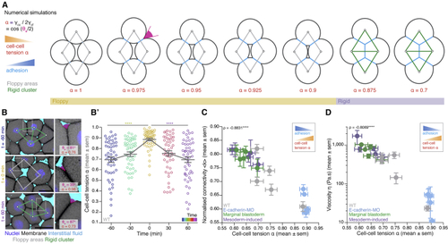
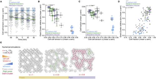
Cell-cell adhesion defines cell connectivity and blastoderm rigidity

(A) Numerical simulations of a mechanical toy model for the morphology of a 4-cell rhombus cluster. Increasing cell-cell adhesion (blue) by decreasing cell-cell tension α (orange) results in contact size expansion and increased connectivity, promoting the emergence of rigid connectivity motifs (green cluster). Contact angle θe (magenta) is used to infer α. Floppy areas are illustrated in gray and rigid areas in green. Yellow- and purple-shaded areas indicate floppy and rigid clusters, respectively (exact values of the α threshold slightly depend on the initial configuration of cells).

(B) Exemplary high-magnification 2D confocal sections at the 1^st–2^nd deep-cell layer of the central blastoderm at consecutive time points overlaid with their rigidity profile during the fluidization/thickening process, with close-ups of exemplary contact angle θe measurements (right, magenta) and calculated cell-cell tension α. Interstitial fluid is marked by dextran, nuclei by H2B-GFP, and membranes by membrane-RFP. Floppy areas are illustrated in gray and rigid areas in green.

(B’) Dot plot of individual cell-cell tension α measurements in the central blastoderm obtained from the experiments shown in (B) overlaid with a line plot of the mean ± SEM as a function of time (color coded) (n = 50 cell-cell contacts, N = 4 embryos per time point).

(C) Plot of normalized connectivity <k> (mean ± SEM) as a function of cell-cell tension α (mean ± SEM) for several experimental conditions during the fluidization/thickening process (for connectivity: central blastoderm of WT n = 55, N = 11; e-cadherin-MO n = 30, N = 6; mesoderm-induced n = 15, N = 3; marginal blastoderm n = 15, N = 3; n, number of blastoderms, N, number of embryos; for cell-cell tension α: n = 50 cell contacts, N = 4 embryos each data point).

(D) Plot of viscosity (mean ± SEM) as a function of cell-cell tension α (mean ± SEM) for the experimental conditions described in (C) during the fluidization/thickening process (for cell-cell tension α: n = 50 cell contacts, N = 4 embryos each data point; for viscosity: central blastoderm of WT n = 53, N = 11; e-cadherin-MO n = 54, N = 6; mesoderm-induced n = 42, N = 6; marginal blastoderms of WT n = 115, N = 9; n, number of embryos; N, number of embryo batches).

Kruskal-Wallis test (B’), ρ Spearman correlation test (C and D). Scale bars: 20 μm in (B).

See also Figure S4.

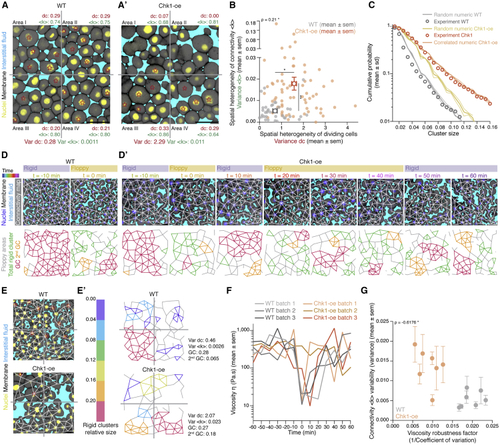
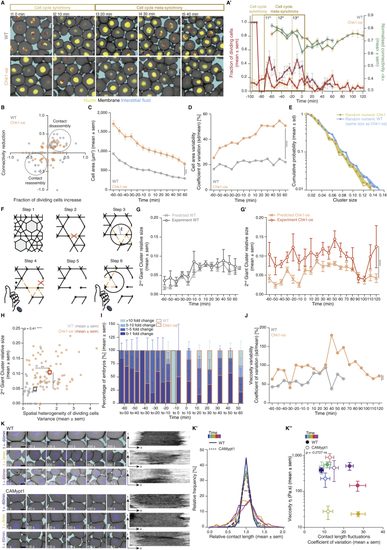
Uniformity in blastoderm rigidity transition relies on meta-synchronous cell divisions generating random cell connectivity changes

(A and A’) Exemplary 2D confocal sections at the 1^st–2^nd deep-cell layer of the central blastoderm of a WT (A) and a Chk1-overexpressing (Chk1-oe, A’) embryo during the last round of meta-synchronous cell cleavages. Interstitial fluid is marked by dextran, nuclei by H2B-GFP, and membranes by membrane-RFP. The Var for the fraction of dividing cells (red stars, dc) and normalized connectivity <k> was calculated between the quadrants.

(B) Plot of the spatial heterogeneity in connectivity as a function of the spatial heterogeneity in the fraction of dividing cells, expressed as the Var in <k> and Var in dc, respectively, between the quadrants (mean ± SEM) shown in (A) and (A’) (WT n = 36 blastoderms, N = 5 embryos; Chk1-oe n = 66 blastoderms, N = 5 embryos; individual Var values are shown in the overlaid dot plot).

(C) Plot of the distribution of rigid cluster sizes p(s) other than the GC for all range of connectivity values in (i) WT and Chk1-oe experimental networks (circles), (ii) simulated random networks with size distribution identical to the experimental ones (WT, shaded gray; Chk1-oe, shaded yellow), and (iii) simulated correlated networks with size distribution identical to the experimental Chk1-oe (shaded orange) (WT n = 103 networks, N = 11 batches, Chk1-oe n = 95 networks, N = 5 batches), showing that Chk1-oe cluster size distribution is wider than the one expected from a model random network, but displays a very good fit if the model network shows spatial correlations in division/bond loss.

(D and D’) Exemplary 2D confocal sections at the 1^st–2^nd deep-cell layer of the central blastoderm of a WT (D) and a Chk1-oe (D’) embryo with overlaid connectivity maps (top) and their rigidity profile (bottom) at different time points during the fluidization/thickening process (color coded), marked as in (A). Floppy areas are illustrated in gray, rigid areas in green, the 2^nd GC in orange, and the GC in red. Yellow- and purple-shaded areas indicate floppy and rigid blastoderms, respectively, as judged by the GC relative size.

(E) Exemplary 2D confocal sections at the 1^st-2^nd deep-cell layer of the central blastoderm of a WT (top) and a Chk1-oe (bottom) embryo, marked as in (D), at a fluidized state with marked mitotic cells (red stars) and overlaid connectivity maps.

(E’) Their rigidity profile is color coded for the size of the rigid clusters (fraction occupied in the total network).

(F) Plot of blastoderm tissue viscosity as a function of time for measurements from 3 independent embryo batches of WT (showing synchronous fluidization) and Chk1-oe (showing heterogeneous phases of fluidization/thickening) embryos.

(G) Plot of normalized connectivity <k> variability, expressed as the Var in normalized connectivity <k> between the quadrants (mean ± SEM) shown in (A) and (A’) as a function of a robustness viscosity factor, expressed as the inverse of coefficient of Var between the viscosity measurements (see Figure S5J) during cell-cycle meta-synchrony.

Kruskal-Wallis test (B), ρ Spearman correlation test (B and G). Scale bars: 50 μm in (A), (A’), (D), (D’), and (E).

See also Figure S5, Table S1, and Video S3.

Temporal analysis of blastoderm viscosity and underlying cellular dynamics, related to Figure 1

(A) Plot of exemplary deformation (d) curves from creep and recovery aspiration experiments in the central blastoderm of sphere stage embryos (t-30min) for different aspiration times and integrated plot of the obtained viscosity values from these experiments, which found to be independent of the aspiration time. The ‘x’ signs indicate the region of the curve where the blastoderm undergoes a viscous deformation and where the slope was used for calculating the viscosity (see STAR Methods for details). Arrowheads indicate the time point of pressure release.

(B) Plot of central blastoderm tissue viscosity (mean ± sem) as a function of the mean squared relative displacement (MSRD) of the blastoderm cells (mean ± sem), during 30min intervals from different starting time points during the fluidization/thickening process (B’). Color-code indicates 30min intervals with dark blue corresponding to viscosity at t-60min and MSRD from t-60min to t-30min, green to viscosity at t-30min and MSRD from t-30min to t0min, yellow to viscosity at t0min and MSRD from t0min to t30min, red to viscosity at t30min and MSRD from t30min to t60min and purple to viscosity at t60min and MSRD from t60min to t90min (for viscosity n = 53 embryos, N = 12 embryo batches; for MSRD n = 26 cell doublets, N = 8 embryos). Statistical tests were performed in comparison to t0min. (B’) Exemplary 2D confocal section at the 1^st-2^nd deep cell layer of the blastoderm at t-60min (left) and color-coded 3D cell trajectories (right) for five representative cells. Nuclei are marked by H2B-GFP and membranes by membrane-RFP.

(C) Plot of central blastoderm tissue viscosity (mean ± sem) as a function of the cell shape index (mean ± sem) (n = 390 cells, N = 3 embryos). Overlaid dot plot shows individual measurements of the cell shape index for each time point. The gray dashed line indicates the theoretical cell shape index value at which a jamming transition is predicted in epithelial tissues. Statistical tests were performed in comparison to t0min. (C’) Exemplary 2D confocal sections at the 1^st-2^nddeep cell layer of the blastoderm marked as in (B’) at t-10min and t0min, with 3 exemplary cell shape index measurements for each.

(D) Plot of central blastoderm tissue viscosity (mean ± sem) as a function of nuclei density (mean ± sem) (n = 103 blastoderms, N = 11 embryo batches). Statistical test was performed in comparison to t0min. (D’) Exemplary 2D confocal sections at the 1^st-2^nd deep cell layer of the blastoderm with marked nuclei by H2B-GFP at t-10min and t0min with indicated number of nuclei (N).

(E) Plot of central blastoderm tissue viscosity (mean ± sem) as a function of cell fraction (mean ± sem) (n = 78 blastoderms, N = 6 embryo batches). Statistical test was performed in comparison to t0min. (E’) Exemplary binary images from the 2D confocal sections shown in (D) with marked interstitial fluid by dextran at t −10min and t 0min with indicated cell fraction (cf.) measurements.

(F) Plot of central blastoderm tissue viscosity (mean ± sem) as a function of cell area (mean ± sem) (n = 652 cells, N = 6 embryos) during the fluidization/thickening process (color-coded for 10min intervals). Statistical test was performed in comparison to t0min. (F’) Exemplary cell area A measurements from the 2D confocal sections shown in (C) with nuclei marked by H2B-GFP, membranes by membrane-RFP and interstitial fluid by dextran, at t-10min and t0min.

(G) Rigidity analysis of an exemplary network. Two rigid clusters (green, red) and a floppy area (gray) are identified. The shaded areas of the network depict potential response to deformation forces that would require no energy cost. Adding a single link can change the overall response of the network to deformation forces due to the sharp increase in the size of the Giant Cluster (GC) (red).

(H) Plot of connectivity < C > (mean ± sem) as a function of cell fraction cf. (mean ± sem) obtained from the same 2D confocal sections of the central blastoderm during the fluidization/thickening process, color-coded for 10min intervals (n = 78 blastoderms, N = 6 embryo batches). (H’) Exemplary binary images from the 2D confocal sections shown in (D) with marked interstitial fluid by dextran and overlaid connectivity maps at t-10min and t0min with indicated cf. and < C > values.

(I) Two exemplary triangular lattices of N = 46, L = 7, one fully connected (top panel) with < C > = 4.9, and the other one partially connected (bottom panel) with < C > 3.6, N, number of nodes, L, side length. Numerical construction of lattices starts with a fully connected lattice of certain L followed by the random removal of links until the desired average connectivity is achieved.

(J) Plots of the linear regime of the response of the lattice against deformations as a function of normalized connectivity for an elastic lattice (left), viscous lattice with bonds half lifetime τ = 2Te (middle) and τ = Te (right), with Te being the simulation time. A permanent displacement of δx = 0.01 a.u. is applied to the top layer of nodes, while the bottom layer remains fixed - (see Figure 1H). The viscosity for viscous lattices is computed from the force exerted by the bottom layer against the deformation. The linear increase of the resistance exerted by the network starts at the critical point of the rigidity percolation (shaded area, predicted rigid regime). Parameters of the simulation are given in STAR Methods.

(K) Dot plot of individual connectivity < C > values obtained from 2D confocal sections of the same blastoderm at the 1^st-2^nd deep cell layer and at the 3^rd-4^thdeep cell layer overlaid with a line plot of the mean ± sem as a function of time (n = 50 blastoderm networks, N = 5 embryos). (K’) Exemplary blastoderm confocal sections (marked as in F) at the 1^st-2^nd(top) and the 3^rd-4^th(bottom) deep cell layer with overlaid connectivity maps and indicated < C > values.

(L) Dot plot of the number of contacts per cell as counted from XY (2D) and XYZ (3D) confocal views (mean ± sem) as a function of time (n = 30 cells, N = 3 embryos for each time point). (L’) Exemplary XY and XZ blastoderm confocal sections marked as in (F’). Purple circle indicates the cell chosen for counting its cell-cell contacts, gray circles indicate neighboring cells in contact to the chosen cell.

Kruskal-Wallis test (B, C), Mann-Whitney test (D-F, H), ρ Spearman correlation (B-F, H). Scale bars, 50 μm (B’, D’, E’, H’, K’), 20 μm (C’, F’, L’).

Rigidity analysis in WT embryos, related to Figure 2

(A) Confocal images of the central blastoderm of an exemplary WT embryo imaged at 1^st-2^nddeep cell layer with nuclei marked by H2B-GFP and membranes by membrane-RFP at consecutive time points during the fluidization/thickening process taken from a time lapse video of a WT embryo.

(B) Same images as shown in (A) with labeled interstitial fluid marked by dextran to reveal the spaces between the cells.

(C) Same images as in (B) with overlaid connectivity maps.

(D) Rigidity analysis of the connectivity maps shown in (C). Floppy areas are illustrated in gray, rigid areas in green, the Giant Cluster (GC) in red and the 2^nd GC in orange.

Experimental manipulations of connectivity, topological rigidity, and tissue viscosity, related to Figure 3

(A) Exemplary 2D confocal sections at the 1^st-2^nddeep-cell layer of the central blastoderm of a control-morpholino (MO) injected embryo with overlaid connectivity maps (top) and their rigidity profile (bottom) at consecutive time points during the fluidization/thickening process. Interstitial fluid is marked by dextran, nuclei by H2B-GFP and membranes by membrane-RFP. Floppy areas are illustrated in gray, rigid areas in green, the Giant Cluster (GC) in red.

(B) Exemplary 2D confocal sections of the central blastoderm of a control-MO and an e-cadherin-MO injected embryo immunostained for E-cadherin.

(C) Plot of E-cadherin protein levels (mean ± sem) as judged by the fluorescence intensity of the immunostaining experiments as a function of time (control-MO, n = 18 embryos; e-cadherin-MO, n = 16 embryos, N = 2 embryo batches).

(D) Exemplary top views of ntl, gsc and wnt11 expression in zebrafish WT and mesoderm-induced embryos at the onset of blastoderm spreading (t0min).

(E) Exemplary 2D confocal sections at the 1^st-2^nddeep-cell layer of the marginal blastoderm of a slb/wnt 11mutant embryo marked as in (A) with overlaid connectivity maps (top) and their rigidity profile labeled as in (A) (bottom) at consecutive time points during the fluidization/thickening process.

(F) Plot of blastoderm tissue viscosity (mean ± sem) as a function of the fraction of the network occupied by the GC (mean ± sem) for the experimental conditions described in Figure 3D (for viscosity: central blastoderm of WT n = 129, N = 11; e-cadherin-MO n = 94, N = 6; control-MO n = 71, N = 6; CAMypt1 n = 66, N = 7; slb/wnt11 f2 mutant n = 54, N = 4; mesoderm-induced WT n = 42, N = 6; mesoderm-induced slb/wnt11 f2 mutant n = 13, N = 3 embryos; marginal blastoderms of WT n = 115, N = 9; slb/wnt11 f2 mutant n = 44, N = 5 embryos; for GC: sample number as described in Figure 3D; n, number of embryos, N, number of embryo batches).

(G) Plot for normalized connectivity < k > (mean ± sem) as a function of time for central blastoderm of WT (n = 103, N = 11), e-cadherin-MO (n = 54, N = 6), control-MO (n = 15, N = 3), CAMypt1 (n = 89, N = 13), slb/wnt11 f2 mutant (n = 10, N = 2), mesoderm-induced WT (n = 15, N = 3) and for the marginal blastoderm of WT (n = 15, N = 3) and slb/wnt11 f2 mutant (n = 15, N = 3) embryos. n, number of networks, N, number of embryos. Grey dashed line indicates the onset of blastoderm spreading.

(H) Plot of tissue viscosity values (mean ± sem) as a function of time for central blastoderm of WT (n = 129, N = 11), e-cadherin-MO (n = 94, N = 6), control-MO (n = 71, N = 6), CAmypt1 (n = 66, N = 7), slb/wnt11 f2 mutant (n = 54, N = 4), mesoderm-induced WT (n = 42, N = 6), mesoderm-induced slb/wnt11 f2 mutant (n = 13, N = 3) and for marginal blastoderm of WT (n = 115, N = 9), slb/wnt11 f2 mutant (n = 44, N = 5) embryos. n, number of embryos, N, number of embryo batches. Grey dashed line indicates the onset of blastoderm spreading.

(I) Plot of the MSRD (mean ± sem) for blastoderm cells of CAMypt1 overexpressing embryos as a function of time (with −60min as reference time point) during the fluidization/thickening process and (I’) an exemplary 2D confocal section at the 1^st-2^nddeep cell layer of a CAMypt1 overexpressing blastoderm marked as in (A) at t-60min with color-coded (for 30min intervals) 3D cell trajectories (n = 10 cell doublets each, N = 3 embryos each).

(J) Exemplary 2D confocal sections at the 1^st-2^nddeep-cell layer of the central blastoderm of an embryo overexpressing CAMypt1 marked as in (A) with overlaid connectivity maps (top) and their rigidity profile labeled as in (A) (bottom) at consecutive time points during the fluidization/thickening process.

(K) Power-law distribution of cluster sizes near the critical point, p(s). The cluster size around the peak of the variance of this distribution, located at around k = 0.68, was computed from an ensemble of lattices with L = 35, N = 1208 (L, side length; N, number of nodes). The blue line shows the slope of a power law with exponent ∼-2.5.

(L) Evolution of variance in rigid cluster size σ2(s) (for clusters other than the GC) along the connectivity values for different lattice sizes (L = 11; 12; 15; 19, N = 116; 139; 218; 352). A clear peak is observed close to the critical point, whose strength grows in size, with the peak displaying a small drift toward higher values than 2/3 of < k > for very small systems due to the increasing role of the boundaries containing nodes with less incident links.

(M) Evolution of σ2(s) as a function of the lattice size N, showing a well-defined dependence σ2(s)∝N. The prediction given in Equation 1 of the STAR Methods, is plotted in blue.

(N) Evolution of the average rigid cluster size < s > (for clusters other than the GC) along the connectivity values for the same lattice sizes as in (L). Contrary to what is observed for σ2(s), < s > has a stable behavior across different connectivity values and displays a convergent behavior as a function of different network sizes. The average rigid cluster size as a function of their normalized connectivity for experimental networks (described in Figure 3F) is plotted with gray circles, showing good agreement with the simulated networks and lacking convergence.

Kruskal-Wallis test (G, H), Mann-Whitney test (C, I). Scale bars, 50 μm (A, B, E, I’, J), 100 μm (D).

Effects of Chk1 overexpression in cellular, topological, and material properties of the zebrafish blastoderm and role of cell contact length fluctuations on tissue viscosity, related to Figure 5

(A) Exemplary high magnification confocal images at consecutive time points during the fluidization/thickening process (10 min interval) of the central blastoderm in WT (top) and Chk1-overexpressing (oe) (bottom) embryos, during synchronous (all the cells in the field of view are dividing at the same time point) and meta-synchronous (only a fraction of the cells is dividing) cell cleavages. Nuclei are marked by H2B-GFP, membranes by membrane-RFP, and interstitial fluid by dextran. Red asterisks indicate mitotic cells, green arrowheads point at contact disassembly in meta-synchronously dividing cells of WT embryos (top) and contact maintenance in asynchronously dividing cells of Chk1-oe embryos (bottom). (A’) Plot of the fraction of dividing cells (mean ± sem) (left axis) from 2D confocal sections of WT (n = 10 blastoderm areas per time point, N = 4) and Chk1-oe (n = 8 blastoderm areas per time point, N = 4) embryos as shown in (A), and of normalized connectivity < k > (mean ± sem) (right axis) from 2D confocal sections as shown in Figures 5D and 5D’ for WT (n = 11 networks per time point, N = ) and Chk1-oe (n = 5 networks per time point, N = 5 embryos) embryos, as a function of time during the fluidization/thickening process, lasting until 60 min in WT and 120 min in Chk1-oe embryos (see STAR Methods for timing difference). Dashed lines indicate the duration of the 11^th, 12^thand 13^thmeta-synchronous cell cycles in WT.

(B) Dot plot of the relative reduction in central blastoderm cell connectivity versus the increase in the fraction of dividing cells within 10 min intervals determined on 2D confocal sections of WT (n = 63 blastoderm areas, N = 5 embryos) and Chk1-oe (n = 94 blastoderm areas, N = 5 embryos) embryos as shown in (A) over the time period directly preceding blastoderm fluidization (1h for WT and 2h for Chk1-oe embryos).

(C) Plot of cell area (mean ± sem) as a function of time during the fluidization/thickening process in WT (n = 652 cells, N = 6 embryos) and Chk1-oe (n = 999 cells, N = 5 embryos) central blastoderms.

(D) Plot of the cell area variability expressed as coefficient of variation (sd/mean) of the data plotted in (C).

(E) Numerical check to discard size and connectivity distribution effects in the discrepancy of Chk1-oe cluster size distribution from its expected random counterpart (yellow curve in Figure 5C). The blue curve is obtained from a re-scaled version of the cluster size distribution found in WT experimental networks, in a way that the average size matches the one found in Chk1-oe experimental networks.

(F) Schematic illustration of the model designed to generate spatially correlated link/bond loss, with correlation length ℓ (at the scale of cell diameter) and correlation probability λ. In step 1, a given state of a lattice of cell contacts is presented. In step 2, a link is chosen at random and removed (orange cross). In step 3, the links in the neighborhood (orange dashed lines) of the removed link (light gray) are identified (black circle), using as a parameter the correlation length ℓ. In step 4, a biased coin is drawn with probability λ to show ‘face’, where ‘face’ removes a link from this neighborhood (orange cross). If ‘tail’ appears, the algorithm goes back to step 2 and the process is restarted. If all the links in the neighborhood are removed (step 5), a biased coin is drawn again (step 6) and if ‘face’ appears, a link that was in the neighborhood is chosen at random and the algorithm goes back to step 3, now taking this randomly chosen link as the starting point. If ‘tail’ appears, the algorithm goes back to step 2. The process starts with a complete lattice and ends when the average connectivity of the networked to be simulated is achieved (see STAR Methods for details).

(G-G’) Plots of the fraction of the network occupied by the 2^nd Giant Cluster (GC) (mean ± sem) in simulated and experimental networks of WT (G) and Chk1-oe (G’) central blastoderms as a function of time during the fluidization/thickening process (WT simulated and experimental, n = 103 networks, N = 11 embryos, each; Chk1-oe simulated and experimental, n = 95 networks, N = 5 embryos).

(H) Plot of the size of the 2^ndGC (mean ± sem) as a function of the spatial heterogeneity in the fraction of dividing cells (expressed as the variance in the fraction of dividing cells between the quadrants shown in Figure 5A, mean ± sem) in WT and Chk1-oe central blastoderms (WT n = 36 blastoderms, N = 5 embryos; Chk1-oe n = 66 blastoderms, N = 5 embryos; individual blastoderm values are shown in the overlaid dot plot).

(I) Plot of the percentage of central blastoderms from different embryo batches undergoing the indicated fold-changes in their viscosity within 10min intervals during the fluidization/thickening process for WT (n = embryos, N = 8 batches) and Chk1-oe (n = embryos, N = 9 batches) embryos.

(J) Plot of the central blastoderm viscosity variability expressed as coefficient of variation (sd/mean) from viscosity measurements of 8 independent WT or Chk1-oe embryo batches.

(K) Exemplary time stills (left) from high magnification confocal time series of cell-cell contact dynamics in WT (top) and CAMypt1 expressing embryos (bottom) and corresponding kymograph (right) during the fluidization/thickening process. (K’) Plot of the relative frequency of cell-cell contact lengths in WT (solid line) and CAMypt1 expressing embryos (dashed line) during the fluidization/thickening process (color coded for 30 min intervals) (n = 10 contacts, N = 4 embryos for each experimental condition and time point). (K’’) Plot of viscosity values (mean ± sem) as a function of contact length fluctuations expressed as coefficient of variation (sd/mean) from the average contact length over a 10 min period in WT (filled circle) and CAMypt1 (clear circle) expressing embryos during the fluidization/thickening process (color coded for 30 min intervals) (for contact length fluctuation: n = 10 contacts, N = 4 embryos for each experimental condition and time point; for viscosity: WT, n = 53, N = 11; CAMypt1, n = 27, N = 7; n, number of embryos, N, number of embryo batches).

Kruskal-Wallis test (G’, H), Mann-Whitney test (C, D, J), ρ Spearman correlation (H, K’’). Scale bars, 20 μm (A) 10 μm (K).