Figure Caption
Figure S3
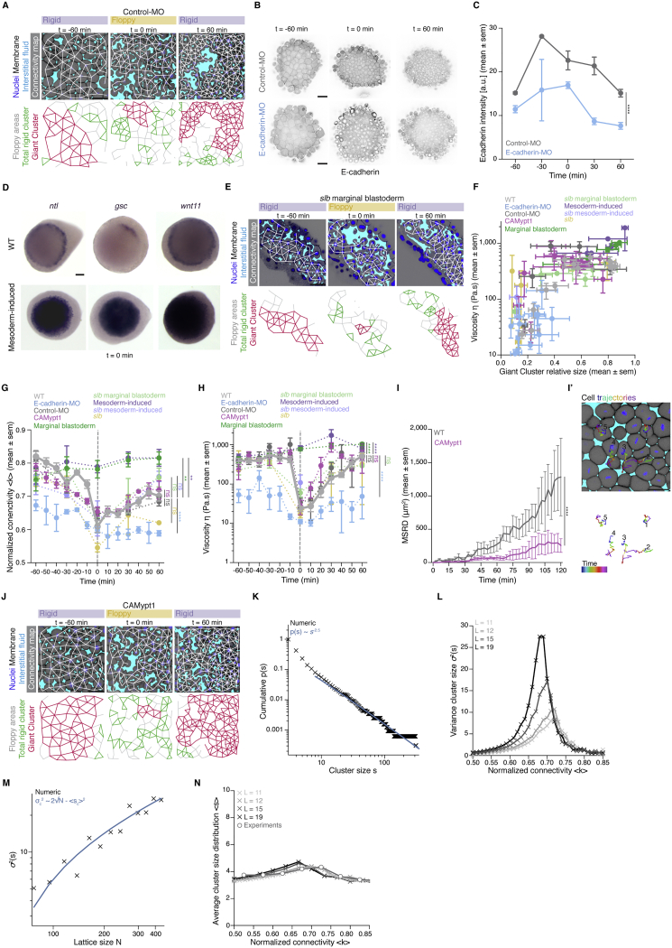
Experimental manipulations of connectivity, topological rigidity, and tissue viscosity, related to Figure 3
(A) Exemplary 2D confocal sections at the 1st-2nddeep-cell layer of the central blastoderm of a control-morpholino (MO) injected embryo with overlaid connectivity maps (top) and their rigidity profile (bottom) at consecutive time points during the fluidization/thickening process. Interstitial fluid is marked by dextran, nuclei by H2B-GFP and membranes by membrane-RFP. Floppy areas are illustrated in gray, rigid areas in green, the Giant Cluster (GC) in red.
(B) Exemplary 2D confocal sections of the central blastoderm of a control-MO and an e-cadherin-MO injected embryo immunostained for E-cadherin.
(C) Plot of E-cadherin protein levels (mean ± sem) as judged by the fluorescence intensity of the immunostaining experiments as a function of time (control-MO, n = 18 embryos; e-cadherin-MO, n = 16 embryos, N = 2 embryo batches).
(D) Exemplary top views of ntl, gsc and wnt11 expression in zebrafish WT and mesoderm-induced embryos at the onset of blastoderm spreading (t0min).
(E) Exemplary 2D confocal sections at the 1st-2nddeep-cell layer of the marginal blastoderm of a slb/wnt 11mutant embryo marked as in (A) with overlaid connectivity maps (top) and their rigidity profile labeled as in (A) (bottom) at consecutive time points during the fluidization/thickening process.
(F) Plot of blastoderm tissue viscosity (mean ± sem) as a function of the fraction of the network occupied by the GC (mean ± sem) for the experimental conditions described in Figure 3D (for viscosity: central blastoderm of WT n = 129, N = 11; e-cadherin-MO n = 94, N = 6; control-MO n = 71, N = 6; CAMypt1 n = 66, N = 7; slb/wnt11 f2 mutant n = 54, N = 4; mesoderm-induced WT n = 42, N = 6; mesoderm-induced slb/wnt11 f2 mutant n = 13, N = 3 embryos; marginal blastoderms of WT n = 115, N = 9; slb/wnt11 f2 mutant n = 44, N = 5 embryos; for GC: sample number as described in Figure 3D; n, number of embryos, N, number of embryo batches).
(G) Plot for normalized connectivity < k > (mean ± sem) as a function of time for central blastoderm of WT (n = 103, N = 11), e-cadherin-MO (n = 54, N = 6), control-MO (n = 15, N = 3), CAMypt1 (n = 89, N = 13), slb/wnt11 f2 mutant (n = 10, N = 2), mesoderm-induced WT (n = 15, N = 3) and for the marginal blastoderm of WT (n = 15, N = 3) and slb/wnt11 f2 mutant (n = 15, N = 3) embryos. n, number of networks, N, number of embryos. Grey dashed line indicates the onset of blastoderm spreading.
(H) Plot of tissue viscosity values (mean ± sem) as a function of time for central blastoderm of WT (n = 129, N = 11), e-cadherin-MO (n = 94, N = 6), control-MO (n = 71, N = 6), CAmypt1 (n = 66, N = 7), slb/wnt11 f2 mutant (n = 54, N = 4), mesoderm-induced WT (n = 42, N = 6), mesoderm-induced slb/wnt11 f2 mutant (n = 13, N = 3) and for marginal blastoderm of WT (n = 115, N = 9), slb/wnt11 f2 mutant (n = 44, N = 5) embryos. n, number of embryos, N, number of embryo batches. Grey dashed line indicates the onset of blastoderm spreading.
(I) Plot of the MSRD (mean ± sem) for blastoderm cells of CAMypt1 overexpressing embryos as a function of time (with −60min as reference time point) during the fluidization/thickening process and (I’) an exemplary 2D confocal section at the 1st-2nddeep cell layer of a CAMypt1 overexpressing blastoderm marked as in (A) at t-60min with color-coded (for 30min intervals) 3D cell trajectories (n = 10 cell doublets each, N = 3 embryos each).
(J) Exemplary 2D confocal sections at the 1st-2nddeep-cell layer of the central blastoderm of an embryo overexpressing CAMypt1 marked as in (A) with overlaid connectivity maps (top) and their rigidity profile labeled as in (A) (bottom) at consecutive time points during the fluidization/thickening process.
(K) Power-law distribution of cluster sizes near the critical point, p(s). The cluster size around the peak of the variance of this distribution, located at around k = 0.68, was computed from an ensemble of lattices with L = 35, N = 1208 (L, side length; N, number of nodes). The blue line shows the slope of a power law with exponent ∼-2.5.
(L) Evolution of variance in rigid cluster size σ2(s) (for clusters other than the GC) along the connectivity values for different lattice sizes (L = 11; 12; 15; 19, N = 116; 139; 218; 352). A clear peak is observed close to the critical point, whose strength grows in size, with the peak displaying a small drift toward higher values than 2/3 of < k > for very small systems due to the increasing role of the boundaries containing nodes with less incident links.
(M) Evolution of σ2(s) as a function of the lattice size N, showing a well-defined dependence σ2(s)∝N. The prediction given in Equation 1 of the STAR Methods, is plotted in blue.
(N) Evolution of the average rigid cluster size < s > (for clusters other than the GC) along the connectivity values for the same lattice sizes as in (L). Contrary to what is observed for σ2(s), < s > has a stable behavior across different connectivity values and displays a convergent behavior as a function of different network sizes. The average rigid cluster size as a function of their normalized connectivity for experimental networks (described in Figure 3F) is plotted with gray circles, showing good agreement with the simulated networks and lacking convergence.
Kruskal-Wallis test (G, H), Mann-Whitney test (C, I). Scale bars, 50 μm (A, B, E, I’, J), 100 μm (D).