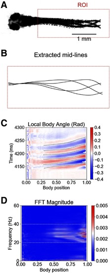
Larval zebrafish tail beat frequency during swimming is mainly between 20 and 40 Hz. A, Four superposed frames recorded during a single swimming episode of a 4-dpf larval fish. The red dotted box is the ROI in which the frame by frame analysis was performed. B, Examples of extracted midlines of the fish body over a swimming episode. C, Heat map of the local body angle amplitude. The fish body was divided into thirty segments from the caudal to the rostral end. The position of the body has been normalized such that the extreme caudal segment is 1.0, and the extreme rostral segment is 0.0. For every frame, the angle of each segment was computed and compared with the resting position. The resulting amplitude was assigned a color, blue for negative angles and red for positive angles. Black dotted lines are used to illustrate successive tail beats. D, For each body segment, a FFT was applied on a swimming episode and the result plotted as a heat map. Note that FFT outputs only positive values. The white dotted box highlights the 20- to 40-Hz range where the frequencies of tail beats reside.

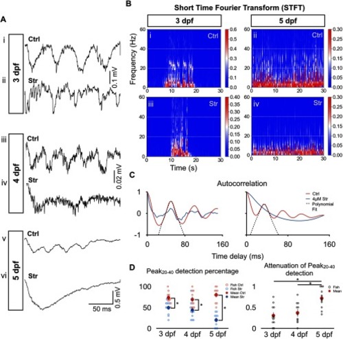
Greater effect of strychnine on tail beat rhythmicity at 5 dpf than at 3–4 dpf. A, Typical extracellular recordings of tail beats during single swimming episodes under control (Ctrl) and 4 μM strychnine (Str) conditions at 3 dpf (Ai, Aii), 4 dpf (Aiii, Aiv), and 5 dpf (Av, Avi). Arrowheads indicate examples of tail beats. Note the relative lack of tail beats at 4 and 5 dpf under strychnine condition (Aiv, Avi). B, Short-time Fourier transform (STFT) of a 30-s-long recording of spinal cord activity under control and 4 μM strychnine conditions at 3 dpf (Bi, Bii) and 5 dpf (Biii, Biv). White dotted lines mark the 20- to 40-Hz frequency range. We can see local maxima in the 20- to 40-Hz range for both 3-dpf plots and the control 5-dpf plot but not for the strychnine-positive 5-dpf plot. C, Example of the autocorrelation function of typical 3- and 5-dpf traces (left and right panel, respectively) under control condition (blue) and strychnine application (red). A polynomial fit (dashed line displays fit to the control trace) was performed to the values of the autocorrelation function within the 20- to 50-ms time delay range. Peak detection was performed to detect the presence of a peak in the polynomial fit within the 25- to 50-ms time delay range, which corresponds to the 20- to 40-Hz frequency range (see Materials and Methods). D, Left, Results from Peak_20–40 detection algorithm for autocorrelation functions under control (blue) and strychnine (red) conditions. Data from somites 4–6 were pooled together. Right, Attenuation of Peak_20–40 detection computed as 1 – (Peak_20–40Strychnine/ Peak_20–40Ctrl). N = 120 episodes (10 per fish, 12 fish) at 3 dpf, and N = 110 episodes (10 per fish, 11 fish) at each of 4 dpf and 5 dpf. Left, Two-tailed paired Student’s t test (at 3-dpf Ctrl-Str, p = 0.0014; at 4-dpf Ctrl-Str, p = 0.0029; and at 5-dpf Ctrl-Str, p = 3 × 10⁻⁵). Right, One-way ANOVA (F_(2,31) = 16.69, p = 1 × 10⁻⁵) followed by two-tailed unpaired Student’s t test (3–4 dpf, p = 0.5283; 3–5 dpf, p = 0.0005; and 4–5 dpf, p = 0.0032); *p < 0.0166, which indicates significance following Bonferroni’s multiple-comparisons correction. Open circles represent the scores of each individual. Solid circles are the averages for every age and condition. Top horizontal bars display result of tests between the two groups at each end of the bars. Error bars display SEM.

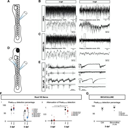
Transition to a SGDR driving tail beats observed in various conditions. A, Schematic of spinalized fish. Fish were cut at the junction between the hindbrain and the spinal cord. B, Upper traces. Typical NMDA induced fictive swimming recording from a 3 dpf (left) and 5 dpf (right) in spinalized fish. Lower traces are magnified views of the dotted boxed regions of the upper traces. C, Same as in B but after addition of 4 μM strychnine to the bath. D, Schematic of the paired ventral root and motor nerve setup. Muscles overlying somites 4–6 were removed. In this diagram, an electrode was attached to a ventral root from either somite 4 or 5 while another electrode was inserted in the muscle cleft of somite 3 to access the motor nerve. E, Representative traces of paired ventral root and motor nerve recordings under control (up) and strychnine (down) conditions for 3-dpf (left) and 5-dpf (right) zebrafish larvae. F, Peak_20–40 detection scores (Fi) and attenuations of Peak_20–40 detection (Fii) for the ventral root and motor nerve recordings in 3- and 5-dpf fish. Open circles represent the scores of each individual. Solid circles are the averages for every age and recording set-up. N = 6 fish; 10 episodes per fish. Error bars represent SEM. For Fi, two-tailed paired Student’s t test (3-dpf root Ctrl-Str, p = 0.8090; 3-dpf nerve Ctrl-Str, p = 0.4149; 5-dpf root Ctrl-Str, p = 0.0053; 5-dpf nerve Ctrl-Str, p = 0.0009). For Fii, two-tailed paired Student’s t test (3-dpf root–3-dpf nerve, p = 0.7093; 5-dpf root–5-dpf nerve, p = 0.4556) and two-tailed unpaired Student’s t test (3-dpf root–5-dpf root, p = 0.0007; 3-dpf nerve–5-dpf nerve, p = 0.0001); *p < 0.0125, which indicates significance following Bonferroni’s multiple-comparisons correction. G, Peak_20–40 detection scores under control and bicuculline (10 μM) conditions in 3-dpf fish. Open circles represent the scores of each individual. Solid circles are the averages for every condition. N = 6 fish; 10 episodes per fish. Error bars represent SEM. Two-tailed paired Student’s t test, p = 0.3739.

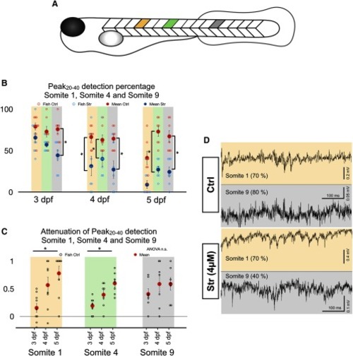
Differential effect of strychnine along the rostro-caudal axis of the zebrafish. A, Schematic of the position at which extracellular recordings were taken: somite 1 (gold), somite 4 (green), and somite 9 (gray). Somites were numbered from 1 to 9 such that somite 1 was the sixth somite rostral to the anus and somite 9 the third one caudal to the anus. B, Results from Peak_20–40 detection algorithm for autocorrelation functions under control (blue) and strychnine (red) conditions for somites 1, 4, and 9. N = 10 episodes per fish in nine fish at every age for somites 1, 4, and 9. Two-tailed paired Student’s t test (3-dpf somite 1 Ctrl-Str, p = 0.0805; 3-dpf somite 4 Ctrl-Str, p = 0.0248; 3-dpf somite 9 Ctrl-Str, p = 0.0065; 4-dpf somite 1 Ctrl-Str, p = 0.0084; 4-dpf somite 4 Ctrl-Str, p = 0.0047; 4-dpf somite 9 Ctrl-Str, p = 0.0141; 5-dpf somite 1 Ctrl-Str, p = 0.0171; 5-dpf somite 4 Ctrl-Str, p = 0.0019; 5-dpf somite 9 Ctrl-Str, p = 0.0090). C, Attenuation of Peak_20–40 detection computed as 1 – (Peak_20–40Strychnine/Peak_20–40Ctrl) for somites 1, 4, and 9. One-way ANOVA for each somite (somite 1, F_(2,22) = 6.286, p = 0.0069; somite 4, F_(2,18) = 7.674, p = 0.0039; somite 9, F_(2,18) = 0.708; p = 0.5057) followed by two-tailed unpaired Student’s t test (somite 1 3–4 dpf, p = 0.0254; somite 1 3–5 dpf, p = 0.0017; and somite 1 4–5 dpf, p = 0.3772; somite 4 3–4 dpf, p = 0.0755; somite 4 3–5 dpf, p = 0.0010; and somite 4 4–5 dpf, p = 0.093). Top horizontal bars display result of tests between the two groups at each ends of the bars. D, Typical traces of dual recordings from somites 1 and 9 from the same fish (3 dpf) before and after strychnine application. Peak_20–40 scores for each respective recording in parentheses; *p < 0.0166, indicating significance with Bonferroni’s multiple-comparisons correction. Open circles represent scores of each individual. Solid circles are the averages for every age and condition. Error bars display SEM.

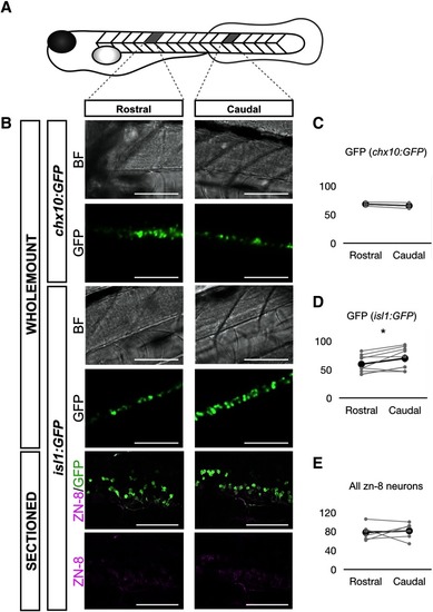
Cell count of sMNs and chx10⁺ spinal neurons in 3-dpf larval zebrafish. A, Schematic of the positions at which Z-stacks were imaged. Counting was performed over two to three somites. B, Representative pictures of targeted rostral and caudal sections, in brightfield (BF) and fluorescent (GFP) conditions for isl1:GFP and chx10:GFP fish in wholemount preparations, and for isl1:GFP fish in sagittal sections of the spinal cord. Scale bars represent 100 μm for wholemount images and 50 μm for section images. C, Count of GFP⁺ cells for the rostral and caudal section in chx10:GFP fish. D, Count of GFP⁺ cells for the rostral and caudal section in isl1:GFP fish. Counts in wholemount and sectioned fish were pooled together. E, Count of zn-8⁺ cells for the rostral and caudal section in isl1:GFP fish. Two-tailed paired Student’s t test (GFP⁺ in chx10:GFP rostral-caudal, p = 0.3196; GFP⁺ in isl1:GFP rostral-caudal, p = 0.0231; zn-8⁺ in isl1:GFP rostral-caudal, p = 0.7274); *p < 0.05, indicating significance. Gray circles are the average of three to four independent counts for each fish. Black circles are the average across all fish. Error bars display SD.

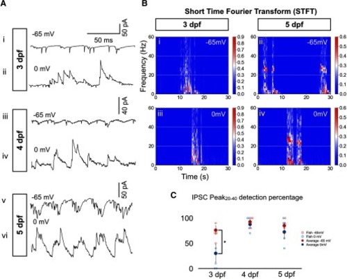
IPSCs mature from arrhythmic at 3 dpf to rhythmic with a frequency close to that of tail beats at 5 dpf during swimming episodes. A, Typical voltage-clamp recordings of MNs during swimming activity at resting (−65 mV) and cation reversal potentials (0 mV) for 3-dpf (Ai, Aii), 4-dpf (Aiii, Aiv), and 5-dpf (Av, Avi) fish. B, Short-time Fourier transform (STFT) of a 30-s-long recording of spinal cord activity under control and strychnine conditions at 3 dpf (Bi, Bii) and 5 dpf (Biii, Biv). White dotted lines mark the 20- to 40-Hz frequency range. We can observe local maxima in the 20- to 40-Hz range for both 5-dpf plots but not for the 0-mV 3-dpf plot. C, Results from Peak_20–40 detection algorithm in the 25- to 50-ms time delay range for autocorrelation functions of each traces at 3, 4, and 5 dpf at −65 mV (blue) and 0 mV (red) holding potentials. N = 10 episodes per sMN in five sMN at 3 dpf, in four sMN at 4 dpf, and four sMN at 5 dpf. Error bars display SEM. Two-tailed paired Student’s t test (3 dpf −65 to 0 mV, p = 0.0139; 4 dpf −65 to 0 mV, p = 0.3910; 5 dpf −65 to 0 mV, p = 0.1942); *p < 0.0166, indicating significance with Bonferroni’s multiple-comparisons correction.

SGDR is preserved in MTZ-treated Tg(dat:NTR-CFP) larvae. Ai, DAPI (white)-labeled horizontal section of Tg(dat:NTR-CFP) zebrafish brain with high-magnification images of the caudal hypothalamus taken from a (Aii) DMSO-treated and (Aiii) MTZ-treated fish. OB = olfactory bulbs, Te = telencephalon, Pr = pretectum, DC = diencephalon, Hc = caudal hypothalamus, LC = locus coeruleus, TeO = optic tectum, Ce = cerebellum, Re = retina. Nomenclature as per Godoy et al. (2015). CFP expression is depicted in magenta. Scale bars = 100 μm (i) and 10 μm (ii). B, Average swimming episode duration (in seconds) calculated for 50 episodes (10 per fish for five fish) at 3 and 5 dpf for DMSO-treated Tg(dat:NTR-CFP) fish and at 5 dpf only for MTZ-treated Tg(dat:NTR-CFP) fish. One-way ANOVA (F_(2,147) = 26.8, p = 1 × 10⁻¹⁰) followed by two-tailed unpaired Student’s t test (3- to 5-dpf DMSO, p = 3 × 10⁻⁹; 3- to 5-dpf MTZ, p = 0.0031; and 5- to 5-dpf MTZ, p = 2 × 10⁻¹⁰); *p < 0.0166, indicating significance with Bonferroni’s multiple-comparisons correction. C, Results from Peak_20–40 detection algorithm for autocorrelation functions of each extracellular recording at 3 and 5 dpf for DMSO-treated Tg(dat:NTR-CFP) fish and at 5 dpf for MTZ-treated Tg(dat:NTR-CFP) fish under control (blue) and strychnine (red) conditions (Ci). Attenuation of Peak_20–40 detection computed as 1 – (Peak_20–40Strychnine/Peak_20–40Ctrl) for each fish. N = 60 episodes (10 per fish for six fish) for 5-dpf Tg(dat:NTR-CFP) fish (Cii). For Ci, two-tailed paired Student’s t test (3-dpf DMSO Ctrl-Str, p = 0.019; 5-dpf DMSO Ctrl-Str, p = 0.0091; 5-dpf MTZ Ctrl-Str, p = 0.0036). For Cii, one-way ANOVA followed (F_(2,26) = 3.98, p = 0.0409) followed by two-tailed unpaired Student’s t test (3- to 5-dpf DMSO, p = 0.0102; 3-dpf DMSO to 5-dpf NTR, p = 0.0398; and 5-dpf WT to 5-dpf NTR, p = 0.8155). Top horizontal bars display result of tests between the two groups at each ends of the bars. Error bars represent S.E.M.

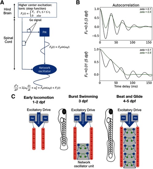
Coupled oscillator model of architectural change from a pacemaker to a network oscillator-based spinal locomotor circuits of developing zebrafish. A, Schematic of coupled oscillators model. Two coupled oscillators: a harmonic oscillator representing a pacemaker (PM) kernel and a damped oscillator representing a half-center network oscillator. The coupling coefficient F₀ represents either the developmental stage or the presence (or absence) of gap-junctions. The damping coefficient models the application or absence of strychnine. The output of the network is read at the output of the half-center. B, Autocorrelation analysis of model output. C, Schematics of the development of spinal locomotor circuits from 3 to 5 dpf. Before 3 dpf, a kernel of IC drives, via gap junctions, two contralateral chains of electrically coupled MNs distributed along the body. Reciprocal inhibition between both sides, which is not illustrated, exists but is not responsible for rhythm generation. After 3 dpf, network oscillators are assembled, first at the caudal end of the spinal cord and then across the length of the spinal cord.