
- Title
-
The neurogenic fate of the hindbrain boundaries relies on Notch3-dependent asymmetric cell divisions
- Authors
- Hevia, C.F., Engel-Pizcueta, C., Udina, F., Pujades, C.
- Source
- Full text @ Cell Rep.
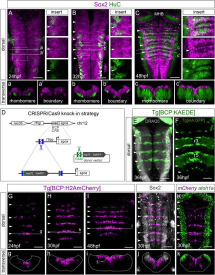
Figure 1. Neurogenesis in boundary cells is delayed compared to neighboring rhombomeres (A–C) Embryos at indicated stages stained with Sox2 (magenta) and HuC (green). Inserts are magnifications of framed regions in (A)–(C), with single or overlayed channels. Note boundaries displaying higher accumulation of Sox2. (a–c, a’–c’) Transverse single-stack views of rhombomeres or boundaries. (D) Scheme depicting the CRISPR-Cas9-based knockin strategy to generate the Tg[BCP:Gal4] fish line. (E and F) Tg[BCP:KAEDE] embryos expressing KAEDE in the hindbrain boundaries. Cell nuclei are in gray. Tg[elA:GFP] expresses GFP in r3 and r5. (G–I, g–i) Spatiotemporal characterization of the Tg[BCP:H2AmCherry] line. White arrows in (i) indicate neuronal derivatives of boundary cells. (J) Tg[BCP:H2AmCherry] embryo stained with Sox2 in gray (boundary cells labeled by the knocked-in reporter; magenta). (K) Double in situ hybridization of Tg[BCP:H2AmCherry] embryos with mCherry and atoh1a. (A–C; E–K) Dorsal maximum intensity projections (MIP) with anterior to the top. (g–k) Transverse views of (G)–(K) as MIP of the indicated boundary (dashed line). Position of boundaries was identified by the morphological bulges (white arrowheads; Calzolari et al., 2014). BCP, boundary cell population; MHB, mid-hindbrain boundary; hpf, hours post-fertilization; ov, otic vesicle; rl, rhombic lip. Scale bar, 50 μm. EXPRESSION / LABELING:
|

Figure 2. Boundary cells undergo neuronal differentiation in a time-dependent manner (A and B) Tg[BCP:H2AmCherry;HuC:GFP] embryos at indicated stages as dorsal MIP with anterior to the top; inserts display single-stack magnifications of the framed regions, with single or overlayed channels. (a and b) Transverse views of (A)–(B) as MIP of the indicated boundary (dashed line). Note that by 48 hpf boundary cells are in the neuronal differentiated domain (see white arrow in insert). White arrowheads in (A)–(B) indicate the position of the hindbrain boundaries. (C) Boxplot showing the increase of differentiated boundary cells (30 hpf [1.14% cells, SD 1.71, SEM 0.38] versus 48 hpf [41.6% cells, SD 5.80, SEM 1.30]; p value t test ∗∗∗p < 0.001). N = 20 boundaries; n = 5 embryos, 4 boundaries per embryo. (D) Spatiotemporal map of the boundary growth showing the position of all cells at the indicated time; annotated boundary cell nuclei (gray dots) displayed on the top of neural tube masks (gray surfaces) and corresponding segmented ventricular surfaces color-coded according to developmental time (33.4 hpf, purple; 36.6 hpf, blue; 40.8 hpf, turquoise; 44.7 hpf, light green); transverse view. (E) Flat representation of the lineage tree of boundary cells color-coded according to the proliferative behavior (blue, dividing; gray, non-dividing) and organized by time of cell division within each category. Each line corresponds to a single cell from the moment of tracking onward, which bifurcates upon cell division. Interrupted lines indicate that cells were lost from the field. X axis, time of embryonic development. (F–F′) Spatial map of a single boundary displaying the regions framed in (D), with annotated boundary cells’ nuclei from (E) as dots in the same color code. t0 = 33.4 hpf (F), tf = 44.7 hpf (F′). (G) Spatial map of a single boundary at tf displaying the region framed in (D), with annotated cell nuclei from progenitors color-coded according to time of division (33.4–36.6 hpf, purple; 36.6–40.8 hpf, turquoise; 40.8–44.7 hpf, yellow). Maps were built after following the lineages of all boundary cells during this time interval, displayed in dorsal (top) or transverse (bottom) views. Analyses in (D)–(G) were performed in ID111219A embryo and backed up with partial analyses of other embryos (Tables S1 and S2 and Figure S3G). BCP, boundary cell population; hpf, hours post-fertilization. Scale bar, 50 μm. |
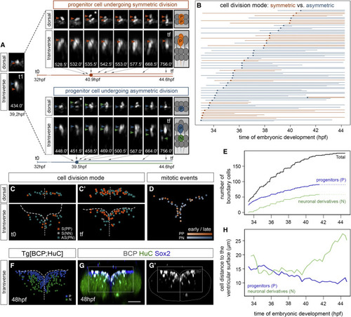
Figure 3. Proliferative boundary progenitor cells undergo both symmetric and asymmetric division (A) Time-lapse stills of a Tg[BCP:H2AmCherry;CAAX:GFP] embryo showing two neighboring progenitor cells undergoing distinct division modes (dorsal and transverse views) color-coded as symmetrical proliferative divisions (PP; orange) and asymmetric divisions (PN; progenitor, blue; neuron, green). White asterisks indicate the corresponding dividing cell. Numbers at the bottom of the transverse stills correspond to the reciprocal minutes of the movie (e.g., t1 = 434.0 min corresponds to a still 7.2 h after the beginning of the movie, 39.2 hpf; tf = 756.0 min corresponds to 12.6 h after, thus 44.6 hpf). The flat lineage diagram depicted underneath each example displays the timeline with the correspondence to the stills. (B) Flat representation of the proliferative boundary cell lineage tree, color-coded according to mode of division (orange, symmetric; blue, asymmetric) and organized by time of division. Each line corresponds to a single cell from the moment of tracking onward that bifurcates upon cell division. X axis displays the time of embryonic development. We did not consider for fate ascription cells tracked for less than 3 h after division if the position of both daughter cells was not clear. An interrupted line means that the cell was lost from the field. (C–C′) Spatial map of a single boundary at t0 = 33.4 hpf (C) and tf = 44.7 hpf (C′) with all annotated nuclei from boundary progenitors shown in (B) color-coded as symmetric proliferative division (orange), asymmetric division (green), and symmetric neurogenic division (gray). Note that only two symmetric neurogenic divisions were found later than 40 hpf (NN, gray cells at tf). (D) Spatial map of a single boundary in transverse view showing the region framed in (G), with the overlay of mitotic events over time (see hues indicating time, early versus late) and color-coded according to cell division mode. Maps were built after following the lineages of all cells of the boundary during this time interval. (E) Graph with the total number of tracked boundary cells (black line), both proliferating and non-proliferating, the boundary progenitors arising from cell division (blue line), and the differentiated neurons derived from asymmetric division (green line), at each time point. Since cell fate could not always be ascribed with enough confidence when cells were tracked for less than 3 h after division, the complete data in the last 3 h of the lineage could not be obtained (see dashed lines from 41.5 hpf onward). (F) Spatial map of a boundary of Tg[BCP:H2AmCherry; HuC:GFP] embryo displaying the ventricular region framed in (G) at tf, with annotated nuclei color-coded according to the final fate (progenitor, blue; neuron, green). Note boundary cells populate the neuronal differentiation domain. (G–G′) Tg[BCP:H2AmCherry] embryos immunostained with Sox2 and HuC at 48 hpf. Scale bar, 50 μm. (H) Graph displaying the average distance to the ventricular surface (0 μm, close, versus 30 μm, far) of the two boundary cell derivatives over time. Note progenitor cells (blue line) become closer to the surface, whereas neuronal derivatives (green line) move away. Analyses in (A)–(E) were performed in ID111219A embryo, with partial analyses of other embryos (Tables S1 and S2). ID111219A and ID260310B were used in (F), and ID111219A and ID111219C were used in (H). |

Figure 4. Boundary cells undergo a switch in Notch-activity (A and B) Tg[BCP:H2AmCherry;tp1:d2GFP] embryos at indicated stages in dorsal view; inserts display single-stack magnifications of framed regions in (A)–(B) with single or overlayed channels. (a and b) Transverse views of the indicated boundary (dashed line). Note that by 48 hpf boundary cells are Notch active (white arrows in inserts). (C) Boxplot showing the switch of Notch-activity in the boundary cells (9.06% at 26 hpf [SD 5.41, SEM 1.21; N = 20 boundaries; n = 5 embryos, 4 boundaries per embryo] to 60.6% at 36 hpf [SD 8.69, SEM 2.7; N = 16 boundaries; n = 4 embryos, 4 boundaries per embryo]; p value t test p < 0.001 [∗∗∗]). (D) Experimental design for loss of Notch function experiments, depicting the hindbrain shape and the treatments with the Notch inhibitor LY411575. (E–H) Transverse views of Tg[BCP:H2AmCherry;HuC:GFP] embryos treated for 6 h at 20 hpf (E–F; DMSO n = 3/3 embryos; LY411575 n = 4/4 embryos) and at 30 hpf (G–H; DMSO n = 4/4 embryos; LY411575 n = 4/4 embryos). Note the increase in the HuC-positive boundary cells (white arrows) when the treatment was after the onset of Notch-activity (H). Scale bar, 50 μm. All inserts display single z stack magnification with single or overlayed channels. (I and J) Boxplots displaying the percentage of differentiated boundary cells (10.81% in DMSO [SD 6.73%, SEM 2.38%] versus 95.63% in LY411575 [SD 1.91%, SEM 0.67%]; p value t test p < 0.001 [∗∗∗]) and the total number of boundary cells (average number per boundary 126 cells in DMSO [SD 25.27, SEM 8.93] versus 106.25 cells in LY411575 [SD 26.30, SEM 9.30]; p value t test p = 0.14 [ns]) at 36 hpf, after DMSO and LY411575 treatment (30–36 hpf). |
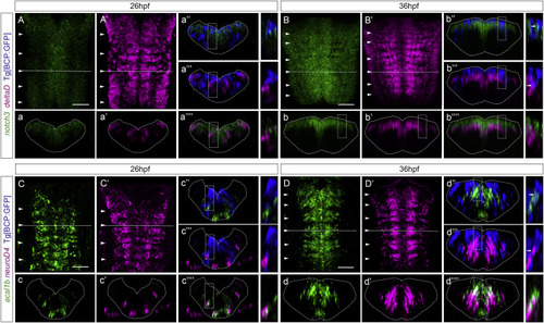
Figure 5. Notch players are expressed in the boundary cells from 36 hpf onward (A–D) Tg[BCP:GFP] embryos, before (26 hpf) and after (36 hpf) the onset of Notch-activity in the boundary cells, were double in situ hybridized with (A–B) notch3 and deltaD and (C–D) ascl1b and neuroD4, followed by GFP staining to detect the boundary cells. (a–a’’’’, b–b’’’’, c–c’’’’, d–d’’’’) Transverse views of the boundary indicated by the dashed line in (A)–(D), displaying staining combinations according to the color-coded labeling. Inserts display magnifications of a single-stack view of the corresponding framed region. Note that notch3 and deltaD staining never overlap. (A–A′, B–B′, C–C′, D–D′) Dorsal MIP with anterior to the top. White arrowheads indicate the position of the hindbrain boundaries. BCP, boundary cell population; hpf, hours post-fertilization. Scale bar, 50 μm. |

Figure 6. Notch3 is crucial for maintaining boundary cells as radial glia progenitors (A–J) Tg[BCP:H2AmCherry;notch3+/+] and Tg[BCP:H2AmCherry;notch3fh332/fh332] embryos were used for the analysis of the (A–D) position of boundary cells and their derivatives (36 hpf, notch3+/+ n = 6/6 embryos versus notch3fh332/fh332 n = 6/6 embryos; 48 hpf, notch3+/+ n = 8/8 embryos versus notch3fh332/fh332 n = 8/8 embryos), (E) differentiated neurons (n = 7/7 embryos), (F–I) Notch-activity (30 hpf, notch3+/+ n = 7/7 embryos versus notch3fh332/fh332 n = 7/7 embryos; 48 hpf, notch3+/+ n = 4/4 embryos versus notch3fh332/fh332 n = 4/4 embryos), and (J) neural progenitor cells (n = 7/7 embryos). Dorsal (A–J) and transverse (a–j) views of the indicated boundary (dashed line). (K–L) Transverse views from Tg[BCP:H2AmCherry;notch3+/+] and Tg[BCP:H2AmCherry;notch3fh332/fh332] embryos labeled with zrf1 (notch3+/+ n = 5/5 embryos; notch3fh332/fh332 n = 7/7 embryos). (M–N) Clonal analysis of radial glia morphology of boundary progenitors. Transverse views of Tg[BCP:Gal4;notch3+/+] and Tg[BCP:Gal4;notch3fh332/fh332] embryos showing plasma membranes in cyan and boundary cell nuclei in white. Note that upon notch3 mutation boundary cells lose the radial glia projection (see inserts). BCP, boundary cell population; hpf, hours post-fertilization. Scale bar, 50 μm. |
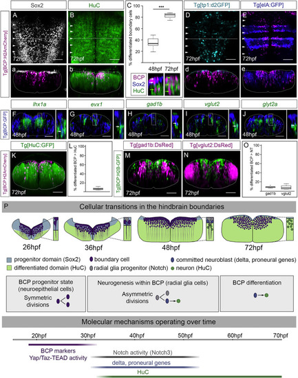
Figure 7. Boundary cells are fated to give rise to neurons (A and B) Tg[BCP:H2AmCherry] embryos immunostained with Sox2 (A) and HuC (B) at 72 hpf. (C) Boxplot displaying the differentiated boundary cells at 48 hpf (34.9%, SD 9.28%, SEM 2.93%) and 72 hpf (82.6%, SD 4.89%, SEM 1.55%; p value paired t test p < 0.001 [∗∗∗]). N = 10 boundaries, n = 5 embryos, two boundaries per embryo. Note magenta cells located in the ventricular zone expressed Sox2 at 48 hpf (white arrows) but not at 72 hpf (HuC cells, green arrows); the displayed region corresponds to the framed area in (b). (D) Tg[BCP:H2AmCherry;tp1:d2GFP] embryos with no boundary progenitor cells displaying Notch-activity at 72 hpf. (E) Tg[BCP:H2AmCherry;elA:GFP] embryos showing rhombomere integrity. (A–B; D–E) Dorsal views with anterior to the top. (a–b; d–e) Boundary transverse views (dashed line). White arrowheads indicate the position of the hindbrain boundaries. (F–J) Tg[BCP:GFP] embryos in situ hybridized with lhx1a (F), evx1 (G), gad1b (H), vglut2 (I), and glyt2a (J) at 48 hpf. Transverse views through r4/r5 or r5/r6; see dorsal views in Figures S6B–S6F. Inserts are magnifications of the corresponding framed regions. Note co-expression of GFP with differentiation factors and neurotransmitters (white arrows in inserts). (K–O) Quantification of the differentiated neurons derived from the boundary cell population. (K, M–N) Tg[BCP:H2AmCherry;HuC:GFP], Tg[BCP:H2B-GFP;gad1b:DsRed], and Tg[BCP:H2B-GFP;vglut2:DsRed] embryos, respectively, as MIP of r4/r5. (L, O) Boxplots with the percentage of differentiated neurons (HuC) (6.5%, n = 7 embryos) and GABAergic and glutamatergic neurons (8.8% GABAergic versus 7.9% glutamatergic; n = 6 embryos each) derived from whole boundaries. BCP, boundary cell population; hpf, hours post-fertilization. Scale bar, 50 μm. (P) Illustration depicting the cellular and functional transitions of the boundary cell population. When neuronal differentiation starts in the hindbrain (26 hpf), boundary cells are progenitors dividing symmetrically (purple). They activate Notch3 signaling (32 hpf), transition to radial glia cells (gray) and undergo asymmetric cell division giving rise to one progenitor (gray) and one committed neuroblast (blue). By 48 hpf, the progenitor domain is reduced; the boundary progenitors still display Notch-activity, whereas the ones committed to the neuroblast lineage differentiate into neurons (green). Finally, the pool of boundary progenitor cells almost extinguishes. Several molecular mechanisms operate over time. Boundary cells are specified at the interfaces between rhombomeres (18–20 hpf) and trigger Yap/Taz-TEAD in response to mechanical stimuli remaining as proliferating progenitors to expand the progenitor pool (Voltes et al., 2019). By 32 hpf, boundary cells are Notch3 active and engage into neurogenesis. Finally, boundary cells most probably undergo direct differentiation, as the differentiation domain dramatically increases at the expense of the progenitor domain. EXPRESSION / LABELING:
PHENOTYPE:
|