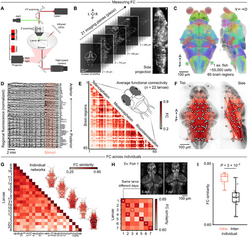
Brain-wide imaging of functional networks in zebrafish larvae. (A) experimental configuration for whole-brain two-photon imaging, light stimulus delivery, and behav-ioral monitoring in tg(elavl3:h2B-GcaMP6s) zebrafish larvae. (B) Five planes highlighted from 21 functional imaging planes at different depths (left); side projection in one examplefish (maximum intensity, right); white arrow indicates the dorsal side; refer to fig. S1 for image scales. (C) centroids of automatically identified neurons from one larva, registered tomapZebrain and mapped into 70 brain regions (pseudocolors; retina/eye is not displayed). (D) Regional fluorescence time series from one representative larva, ordered from ante-rior to posterior regions; a pink rectangle highlights a period of dark-flash visual stimuli. (E) Group-averaged Fc matrix (n = 22 larvae), ordered from anterior to posteriorregions. (F) network visualization of group-averaged Fc, using the same color map as the previous panel; nodes represent brain region centroids, and bottom quartile Fc edges arenot displayed; network edges are mirrored across both hemispheres for visualization. (G) Functional network similarity across larvae, ordered from the most globally similar to themost globally dissimilar individual; five example individual networks are plotted on the right. (H) Functional network similarity of seven larvae imaged on consecutivedays; similarity scores are averaged across both temporal directions, from dataset 1 to dataset 2 and vice versa; white asterisks denote maximal similarity values on each row.(I) network similarity scores are significantly higher when comparing individuals to themselves [diagonal values from matrix in (h)] rather than different individuals [off-diagonalvalues from matrix in (h)] (P = 3 × 10−5, t test). A, anterior; P, posterior; v, ventral; d, dorsal; L, left; R, right.

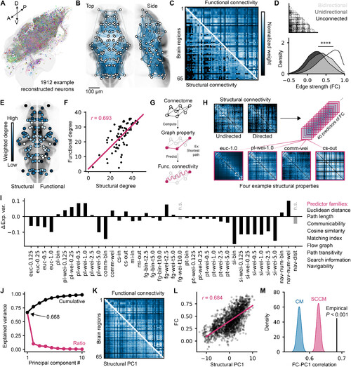
Structure- function coupling of zebrafish brain networks. (A) 3d rendering of 1912 reconstructed neurons generated on mapZebrain.org. (B) Mesoscopic Scoverlaid on brain anatomy; edge weights are color mapped with the next panel, and bottom quartile edges are not displayed. (C) Undirected Sc matrix compared withFc; matrices are arbitrarily scaled for visualization. (D) distributions of individually sampled Fc values from edges that have either bidirectional, unidirectional, or no un-derlying structural connections (one-way AnOvA, F = 5048, P = 0). (E) Functional and structural node degrees with arbitrary rescaled values for visualization; structuraldegrees are displayed on the left hemisphere, and functional degrees are displayed on the right. (F) Linear regression between structural and functional degrees (Pearson’sr = 0.693). (G) depiction of the Fc modeling approach used in following panels; properties of the structural network, such as the shortest path between two nodes, areused to predict Fc. (H) Four example matrices from an array of 40 graph properties used as predictors of Fc in this study. (I) Fc variance explained by each of the predictors,subtracted by the variance explained by Sc; predictor families are indicated on the right, in the same order as the bar chart labels. n.s., not significant. (J) Relative (red) andcumulative (black) variance explained by each Pc derived from the set of predictors. (K) Structural Pc1 compared to Fc; matrices are arbitrarily scaled for visualization.(L) Linear regression between upper triangle values of structural Pc1 and Fc (Pearson’s r = 0.684). (M) null distributions of structural Pc1 correlations derived from null Scmatrices (1000 matrices per distribution, empirical P < 0.001).

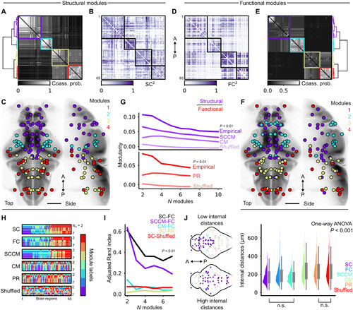
Structural and functional modules are spatially overlapped at multiple hierarchical levels. (A and D) Module coassignment probability matrices, hierarchi-cally clustered using Ward’s linkage (for Sc and Fc, respectively); four modules are chosen arbitrarily as an intermediary hierarchical level for visualization. (B and E) con-nectivity matrices, reordered by modules according to the previous panels (Sc and Fc, respectively); colors are mapped to squared edge weights for better contrast.(C and F) Brain region centroids colored by module membership (Sc and Fc, respectively); scale bars, 100 μm. (G) Structural and functional modularity at different hierar-chical levels, compared against various null models. Sc modularity curves are plotted above (purple), and Fc curves are below (red); 99th percentiles of null distributionsare plotted for null models. SccM, spatially constrained configuration model; cM, configuration model; PR, phase-randomized time series (see Materials and Methods).(H) Module identity vectors plotted at different hierarchical levels, for both empirical data and null models; N m denotes the number of modules; representative labels areshown for each null model. (I) Adjusted Rand index computed on pairs of module labels from the previous panel at different hierarchical levels; 99th percentiles of nulldistributions are plotted. (J) Left: visual examples of spatially compact (top) versus distributed (bottom) modules. Right: Boxplots of pairwise internal distances betweenregions belonging to the same modules, compiled across all hierarchical levels; all distributions are different with the exception of two comparisons, as indicated belowthe figure (one-way AnOvA, P < 0.001, followed by tukey’s post hoc test for pairwise comparisons).

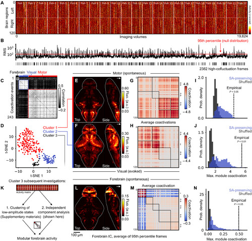
Mesoscopic coactivation patterns coincide with the modular organization of SC. (A) Raster plot of z- scored regional activity across 22 larvae. Left and righthemispheres are plotted in the upper and lower halves, respectively. (B) Root-mean-square (RMS) of regional coactivation values for each of the corresponding frames in(A); the red line indicates a statistical threshold for high coactivation events (P < 0.05, false discovery rate fixed at α = 0.05 using the Benjamini-hochberg procedure).(C) correlation matrix of 243 detected events, separated into three clusters that are illustrated in the following panel. (D) t-Sne projection of 243 high-amplitude events,with three clusters identified using density-based clustering. (E and F) Raw data projections of the two main clusters, coregistered and averaged across larvae (n = 22);top; high- amplitude motor events; bottom: high- amplitude visual responses to dark stimuli; contrast is adjusted after averaging (see Materials and Methods). a.u., arbi-trary units. (G and H) Average coactivation matrices of the two main clusters, reordered according to four structural modules; statistical significance of module coactiva-tions is indicated on right matrix borders. (I and J) null distributions of maximal module coactivation values in SA-preserving and SA-breaking surrogates; dashed linesindicate empirical coactivation values. (K) two independent analyses recover modular forebrain activity that was weakly detected as cluster 3 in the previous clusteringanalysis. (L) Averaged raw fluorescence from frames corresponding to the 95th percentile of forebrain ic activity. (M) Average coactivation matrix of frames belonging tothe 95th percentile of forebrain ic activity. (N) null distributions of forebrain modularity, similar to (i) and (J).

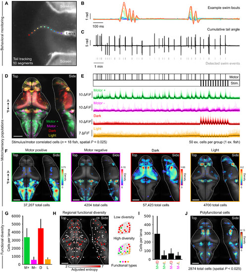
Identification of sensorimotor neuronal populations. (A) example camera frame from high-speed monitoring of a head-restrained larva with tail tracking points.(B) Angular time series of 10 tail segments displaying two successive swimming events; colors correspond to tracking points on the previous panel. (C) cumulative tailangle of one larva over a full experiment, with detected swimming events below. (D) Overlapped densities of motor-positive, motor- negative, dark-responsive, and light-responsive cells, projected on the mapZebrain template brain (n = 18 larvae, spatial) P < 0.025. (E) top; Motor and stimulus event vectors. Bottom: 50 example cells perfunctional category (color traces) with average population activity (black traces). (F) individual cell densities from (d); the color map represents arbitrary spatial densityunits, relative to the maximum density observed in dark-responsive cells; the number of cells aggregated across animals and contributing to each distribution is indicatedbelow each panel; spatial P < 0.025. (G) number of cells per functional category per larva; error bars indicate Sd; statistical comparisons are avoided due to slight meth-odological differences between motor and visual cell identification (see Materials and Methods). (H) Left: Regional measure of functional diversity using adjusted Shannonentropy; nodes reflect region centroids, and node sizes are redundant with the color map. Right: Schematized examples of low and high diversities in a brain region.(I) number of overlapping cells for each nonorthogonal pair of functional categories per larva; error bars indicate Sd. (J) Spatial density of polyfunctional cells detectedacross all animals, spatial P < 0.025. A, anterior; P, posterior; M+, motor positive; M−, motor negative; d, dark; L, light. Scale bars, 100 μm.

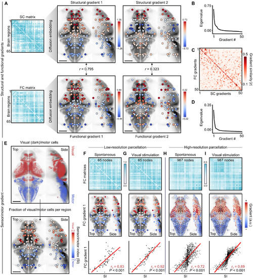
Regional sensorimotor functions coincide with the main functional gradient. (A) top: Sc matrix and its first two diffusion gradients, with nodes denoting brainregion centroids. Bottom: Fc matrix and its first two diffusion gradients. (B) eigenvalues of the first 50 structural diffusion gradients. (C) Absolute correlation ∣ r ∣ betweenthe first 50 Sc and Fc gradients; functional gradients are reordered to optimally match the structural gradients. (D) eigenvalues of the first 50 functional gradients. (E) top:dark and motor-positive neuron centroids from Fig. 5, in red and blue, respectively. Bottom: Sensorimotor index of each brain region. (F) top: Fc matrix under spontane-ous conditions. Middle: First Fc gradient of the corresponding matrix above. Bottom: correlation between sensorimotor index (Si) and first Fc gradient. r s denotes theSpearman correlation coefficient, and P values are obtained through SA-preserving permutations (1000 permutations). (G) Similar to the previous panel, except with Fccomputed while including visual stimuli. (H) Similar to the previous panel, except with high-resolution Fc computed from spontaneous activity. (I) Similar to the previouspanel, except with high-resolution Fc computed while including visual stimuli. Scale bars, 100 μm.

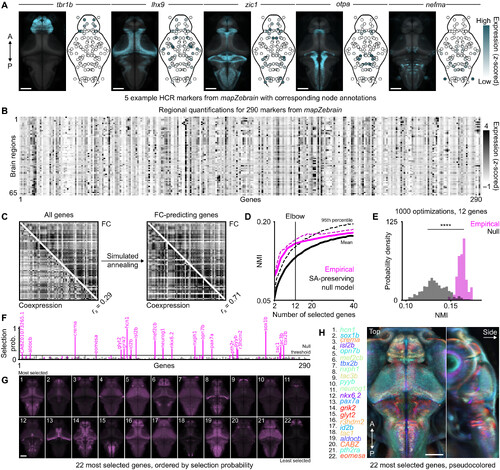
Gene coexpression predicts FC. (A) Five example fluorescence in situ hybridization markers from mapZebrain (left: top view, 90th percentile projections), withcorresponding regional annotations (right: in black outlines); intensities are scaled arbitrarily per gene for visualization. (B) Regional gene expression matrix; each row(brain region) is z-scored independently. (C) Left: cGe matrix across all 290 genes, compared with the Fc matrix; r s denotes the Spearman coefficient. Right: cGe matrix of12 optimized genes obtained through simulated annealing, compared with Fc. (D) Average (full lines) and 95th percentile (dotted lines) of optimized nMi between cGeand Fc for varying numbers of genes used in simulated annealing runs; pink curves correspond to empirical gene sets, whereas black curves correspond to spatiallyshuffled genes; a vertical line indicates the elbow of the average empirical curve; 1000 optimization runs per number of genes. (E) nMi distributions at the predeterminedelbow point for empirical and null optimization results using 12 genes (P < 0.001, t test). (F) Selection frequency of each gene across 1000 simulated annealing runs; pinkbars correspond to empirical genes, whereas black bars correspond to spatially shuffled gene datasets; a horizontal bar denotes a selection threshold, with significantgene names indicated above. (G) 90th percentile intensity projections of 22 significant gene markers; gene names are indicated in the next panel, ordered by selectionprobability (left to right, top to bottom). (H) Overlap of 22 pseudocolored gene markers; pixelwise color contrast is used to highlight the most prominent genes at eachlocation; colors are used to accentuate the global patterns, rather than to precisely distinguish individual genes (which are displayed separately in the previous panel).A, anterior; P, posterior; SA, spatial autocorrelation. Scale bars, 100 μm.