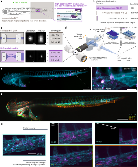
a, Schematic of the field of views of low- (brown) and high-resolution (violet) light-sheet microscopy modalities to image biological processes across scales. b, Calculations of the duration and resulting data sizes for imaging a 2.5-day-old zebrafish larva in one fluorescent channel with high-resolution imaging using axially swept light-sheet microscopy (ASLM), low-resolution imaging and a multiscale imaging approach that captures the whole organism and one selected region of interest with high-resolution. c, Schematic top-view light-sheet profiles of dual-sided multidirectional selective plane illumination microscopy (SPIM) (top, brown) for low-resolution imaging and single-sided ASLM for high-resolution imaging (bottom, violet), with the dark blue arrow indicating the scan direction of the thin ASLM light-sheet (left). Representative images of 0.2-μm fluorescent nanospheres for both modalities (middle). PSF values measured with MetroloJ (n = 20 for each modality) (right). d, Simplified rendering of the multiscale microscope. The low- and high-resolution modalities share the same illumination and detection objectives. In the detection path, a motorized flip mirror selects either the low-resolution or the high-resolution detection path. e, Representative images from the multiscale microscope displaying a 2.5-day-old zebrafish larva (cyan, vascular marker Tg(kdrl:Hsa.HRAS-mCherry); magenta, macrophage marker Tg(mpeg1:EGFP)) xenografted with U-2 OS osteosarcoma cells (white). Low-resolution image of the whole zebrafish larva (left). Zoom in to boxed image to compare the high-resolution image acquired with ASLM (bottom left) to the mSPIM image (top right) (right). f, Representative low-resolution stills from a time-lapse imaging experiment of zebrafish larva expressing the vascular marker Tg(kdrl:Hsa.HRAS-mCherry) are overlaid onto each other, with the color indicating imaging time (starting at 3 days after fertilization). This highlights sample movement and growth over the observation window and the shift of a region of interest over time (boxed region). g, High-resolution imaging with a static, pre-defined imaging volume within the microscope coordinate system (top) and self-driving microscopy (bottom). Same color scheme as in e. Scale bars, 0.5 μm (c); 250 μm (left), 60 μm (right) (e); 250 μm (f); 50 μm (g). FOV, field of view.

a, Multiscale imaging of a SUM159 breast cancer cell spheroid embedded into a collagen matrix (Supplementary Videos 1 and 2) with the low-resolution modality shown on top and the high-resolution modality on the bottom. The spheroids consisted of a 1:1 mixture of cells expressing the actin marker Lifeact-GFP (cyan) and Lifeact-mCherry (magenta). Boxed region on top indicates the location of the high-resolution region on the bottom. The white arrowhead points at a cell division at the invasive front. b, Multiscale imaging of zebrafish gastrulation with cells expressing the histone marker Tg(h2afva:h2afva-GFP), starting at around 6 h after fertilization (Supplementary Videos 3 and 4). Low-resolution imaging (on top) captured the entire zebrafish embryo (color scale, depth of data in 3D volume from 0 to 450 μm), while the high-resolution imaging (bottom) enabled near-simultaneous imaging of cell division (yellow arrowheads), including sister chromatid separations. c, Multiscale imaging of human breast cancer cells MDA-MB-231 expressing F-tractin-EGFP (left, magenta; right, grayscale) in situ in a larval zebrafish xenograft model (Supplementary Videos 5 and 6). The cancer cells were xenografted at 2.25 days post-fertilization into a zebrafish larvae expressing the vascular marker Tg(kdrl:Hsa.HRAS-mCherry) (cyan). Cell-spreading patterns as imaged in the low-resolution mode are shown on the left, and a 3D rendering of the high-resolution data is shown on the right. The white arrowhead points at a network of protrusions. Scale bars, 150 μm (top), 20 μm (bottom) (a); 200 μm (top), 30 μm (bottom) (b); 300 μm (left); 40 μm (right) (c)

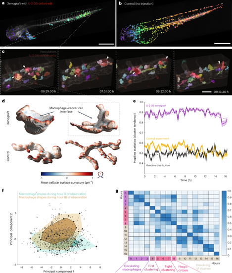
a, Low-resolution, 3D rendering of a zebrafish xenograft with U-2 OS osteosarcoma cancer cells (red), segmented macrophages (color scale, violet to green from head to tail) and a vasculature label, Tg(kdrl:Hsa.HRAS-mCherry) (gray). Boxed region indicates the location of high-resolution region in c. b, Low-resolution, 3D rendering of a zebrafish larva without xenograft (control) with segmented macrophages (color scale, violet to red from head to tail) and a vasculature label, Tg(kdrl:Hsa.HRAS-mCherry) (gray). c, 3D rendering of high-resolution stills with segmented macrophages (in color), U-2 OS cancer cells (red, white arrowhead) and vasculature (gray). Boxed region indicates individual macrophage highlighted in d. d, 3D renderings of individual macrophages from the high-resolution data of xenograft experiment (top) and control (bottom). Color indicates mean cellular curvature. e, Hopkins statistics (10% sampling, dimensionality d = 3) to analyze macrophage cluster tendency inside a zebrafish. A higher number indicates a higher cluster tendency with U-2 OS xenograft data in violet, control data (no xenograft) data in yellow, and a simulation of a randomized, uniform distribution in black. Data are displayed as mean ± 95% CI (n = 350 iterations for Hopkins statistic calculation). The dashed line indicates the moving average of ten time points. f, Global morphological feature analysis of macrophage shapes (gray points, n = 825 cells) from the high-resolution data of the U-2 OS cancer cell xenograft experiment over time, displayed in a PCA plot. Bagplots of all macrophage shapes in the first hour (hour 0; turquoise) and hour 16 (brown) of observation are overlaid. The bagplot consists of the Tukey median (cross), an inner polygon (darker color) that contains the 50% observations with largest Tukey depth and the outer polygon (lighter color) with all data excluding outliers. g, Change of macrophage shapes over time; all macrophage shapes within an hour of observation were compared to macrophage shapes at different hours by applying a permutation test (one-sided, no adjustment for multiple comparison, n = 3,000 iterations) using the Tukey median as a metric. The resulting P values were plotted as a heat map. Scale bars, 500 μm (a and b) and 50 μm (c).

We introduce two designs for a multiscale microscope with dual-sided illumination (gray), a remote focusing unit (light gray) and detection with two resolutions (orange): a one design operating with cylindrical lenses and using a motorized slit, and b one design using Powell lenses, where no motorized slit is required (Supplementary Note 1). The microscope hardware comfortably accommodated several samples in one experiment, mounted in low melting agarose within fluorinated ethylene propylene (FEP) tubes. Abbreviations are as follows: 4 different lasers (LS1-LS4), dichroic beamsplitters (DC), 4x telescope (T1, f1 = 50 mm, f2 = 200 mm), pinhole (PI), halfwave plate (λ1/2), polarized beamsplitter cube (PBS), motorized flip mirror (FM), two cylindrical lenses (CT, f1 = 25 mm, 100 mm), vertical slit (VS), resonant galvanometer (RM), low-resolution cylindrical lens (Cl, f = 200 mm), tube lens (TLi, f = 100 mm), illumination objective (IL, NA 0.4), telescope (T2, 5x), motorized vertical slit (mVS), high-resolution cylindrical lens (Ch, f = 50 mm), tube lens (Trm, f = 200 mm), remote focusing objective (RF), a quarterwave plate (QWP), telescope (T3, f1 = 200 mm, f2 = 75 mm), 10° Powell lens (P), f = 30 mm lens (L1), f = 60 mm lens (L2), f = 400 mm lens (L3), voice coil with a mirror (VCM), LED illumination (LED), 20x NA1.0 detection objective (DL), filter wheel (FW), 100 mm tube lens (TL1), 500 mm tube lens (TL2).

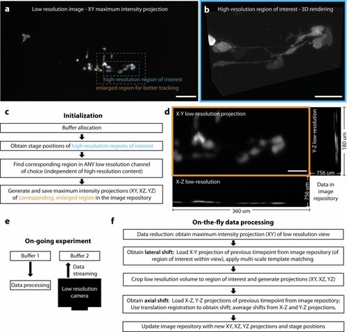
a Low-resolution maximum intensity projection of MDA-MB-231 breast cancer cells, labeled with F-tractin-GFP, in the zebrafish tail. Insets depict a high-resolution region of interest (blue, panel b) with its corresponding, enlarged (1.5x in both lateral dimensions) region used for better tracking. b 3D rendering of the high-resolution region of interest. c Schematic of the steps required for initialization of the region tracking algorithm. d X–Y, Y–Z, X–Z low-resolution maximum intensity projections saved in the image library at initialization, and each subsequent time point / update step. e Schematic of simultaneous data processing and acquisition (data streaming), enabled by a custom buffer architecture using shared memory arrays and tools from the concurrency tool library by Thayer, York et al. f Schematic of the pipeline for the update step to calculate on-the-fly the lateral and axial shifts for region tracking. Scale bar lengths are as follows: a 150 μm, b,d 50 μm.

a Selected maximum intensity projections of transmission images of the larval zebrafish tail over 11 hours of observation, starting at 2.5 days post-fertilization. The blue dashed line indicates the tip of the vasculature at the end of the tail, growing around 100 μm over the 11 hours window of observation (blue arrows). b Despite this growth, self-driving microscopy kept the vascular region of interest in focus over the observation window. Maximum intensity projections of the corresponding high-resolution region showcase details of the outgrowth of a single vessel (white arrowhead) with subsequent anastomosis (white arrows) with a neighboring vessel, including positioning of endothelial nuclei (asterisk). The vasculature was labeled with Tg(kdrl:EGFP). c Maximum intensity projection of the entire field of view of the low-resolution acquisition at start of the time-lapse imaging, with the inset highlighting the region used for tracking. d Representative X–Y, Y–Z, X–Z maximum intensity projections used in the region tracking algorithm. Scale bar lengths are as follows: a, c, d 150 μm; b 50 μm.

a Schematic of our in vivo zebrafish xenograft assay to study immune cell–cancer cell interactions in situ. Firstly, human cancer cells were cultured and modified as desired, for example, by expressing a fluorescent marker to label the cells. Secondly, cells were harvested and injected near the common cardinal vein (CCV) into the yolk of zebrafish larvae (violet arrow). Then, xenografts were imaged on our self-driving, multiresolution microscope, and subsequent analysis allowed visualization and quantification of cell spreading, cell–cell interactions, and cell morphological changes. b Low-resolution mSPIM images captured the distribution of macrophages (Tg(mpeg1:EGFP), top: magenta, bottom: grayscale image) in the entire zebrafish larvae after xenografting U-2 OS osteosarcoma cells (pVimentin-PsmOrange label, top: white, bottom: bright white). For tissue context, zebrafish also expressed the vascular marker Tg(kdrl:Hsa.HRAS-mCherry) (top: cyan). The image highlights how macrophages clustered around sites with cancer cells (Supplementary Movie 7). c In contrast, zebrafish without xenografts (control) displayed a uniform distribution of macrophages (Tg(mpeg1:EGFP), top: magenta, bottom: grayscale image) across the entire zebrafish embryo (top: vascular marker Tg(kdrl:Has.HRAS-mCherry in cyan). d The self-driving feature of the microscope enabled high-resolution imaging of selected cancer colonies in the zebrafish tail over many hours by keeping it in focus. Frequently, we observed how zebrafish macrophages (Tg(mpeg1:EGFP), top: magenta, bottom: gray) attached to the U-2 OS cancer cells (pVimentin-PsmOrange label, top and bottom: green), and phagocytosed them (Supplementary Movie 7, 8). Scale bar lengths are as follows: b,c 500 μm; d 50 μm.

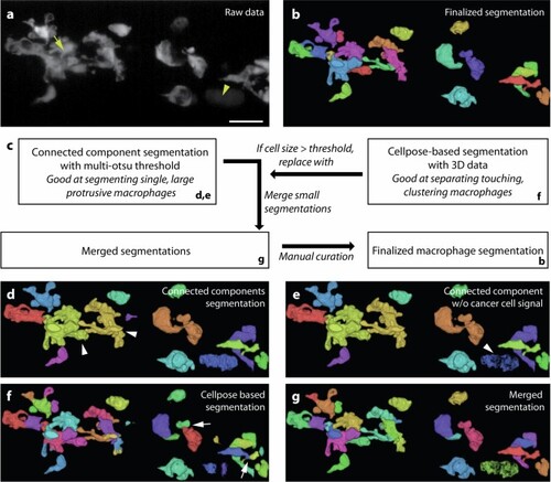
a Maximum intensity projection of a 3D volume in the caudal hematopoietic tissue visualizing zebrafish macrophages, labeled with Tg(mpeg1:EGFP)62, after xenografting human U-2 OS cells into the zebrafish larvae. As the cancer cells (yellow arrowhead) were labeled with a psmOrange fluorophore, there was bleed-through into the macrophage channel (GFP). Moreover, macrophages tended to cluster around cancer cells and at locations where cancer cells resided before they were phagocytosed by macrophages (yellow arrow). b 3D rendering with Fiji’s 3D viewer to display the final segmentation by the proposed workflow. c Schematic of the segmentation workflow. d We initially segmented the data with multi-Otsu thresholding and connected component labeling. This segmented individual macrophages well, for example in the control experiment (without xenografts) or at the beginning of the xenograft experiment. However, it could not separate touching macrophages (white arrowheads). e To clean up the segmentation, we first removed the cancer cell signal (white arrowhead) from the segmentation. f To separate clustering macrophages, we constructed 3D consensus segmentation from Cellpose-2D46 segmentations computed in orthogonal x–y, x–z, y–z views of the original raw data. While this segmentation separated clustering macrophages, it was observed to split individual macrophages into smaller fragments (white arrows) when the macrophages show extensive cytoplasmic extensions of several tens to hundreds of microns. g We merged the connected component segmentation and the Cellpose-based segmentation by replacing connected volumes that exceeded a defined threshold with the Cellpose-based segmentation. Moreover, we merged connected volumes that were below a certain threshold with neighboring volumes. Subsequent manual curation further cleaned up the segmentation of macrophages to obtain the finalized segmentation b. Scale bar lengths are as follows: a 30 μm.