Figure 1. Principle of DAOSLIMIT

(A) Schematic of the sLFM system for high-resolution spatial-angular measurements.

(B) Illustrations of DAO. Different angular components can be manipulated in postprocessing for 3D reconstruction and aberration corrections.

(C) Illustrations of the periodic scanning process and pixel realignment. Different colors correspond to specific galvo positions (indicated by the arrows) with a period of 9 for 3 × 3 scanning. The sensor pixels with the same relative position to the center of each microlens belong to the same angle. Images at different scanning positions can be realigned together to increase spatial sampling for 3D reconstruction with tiled aberration corrections digitally.

(D) Comparisons between the PSFs, OTFs, and simulated imaging results of LFM, sLFM, and WFM with a 63×/1.4 NA oil-immersion objective and WFM with a 63×/0.2 NA air objective at a center wavelength of 525 nm. The simulated sample is a high-frequency sinusoidal pattern with a period of 1.3 μm, as shown in the bottom right corner. To show the highest contrast, the sample is placed at the native focal plane for WFM and 1 μm away from the focal plane for LFM and sLFM.

(E) Illustrations of the time-weighted algorithm. High-resolution time-lapse data can be obtained by applying inverse distance weighting in the xyt domain with a sliding window.

(F) Comparisons between the reconstructed results (MIP) of DAOSLIMIT with and without the time-weighted algorithm.

Scale bars: 5 μm, 2 μm⁻¹ (D) and 10 μm (F).

See also Figures S1 and S2 and Video S1.

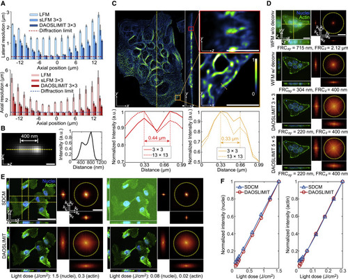
Figure 2. Resolution and SNR characterization of DAOSLIMIT

(A) Boxplots of the lateral and axial resolutions of LFM, sLFM (DAO off), and DAOSLIMIT at different axial positions with 63×/1.4 NA oil-immersion objective. The resolution is estimated by the FWHMs of the intensity profiles with a Gaussian fit for 100-nm-diameter beads distributed in 1% agarose (n = 300 beads, 20 beads per plane). Error bars represent SD.

(B) MIP of two beads in yz plane obtained by DAOSLIMIT at the focal plane with a cross-section profile. We imaged the same bead at two axial planes separated by 400 nm and added the images to create virtually spaced beads.

(C) Orthogonal MIPs from 12-μm-thick slabs of MCF10A cells labeled with microtubules imaged by DAOSLIMIT (3 × 3 scanning), with normalized profiles of the marked lines.

(D) Orthogonal MIPs from 16-μm-thick slabs of HeLa cells labeled with actin (green) and nuclei (blue), which were obtained by WFM (90 axial slices at 200-nm steps), WFM with 3D deconvolution, and DAOSLIMIT with 3 × 3 and 5 × 5 scannings. The Fourier transforms of the MIPs are shown with estimated resolutions by FRC. Throughout the figure, the yellow dashed circles correspond to the Abbe diffraction limit of the objective.

(E) Orthogonal MIPs and corresponding Fourier transforms of the MCF10A cells with actin (green) and nuclei (blue) labeling imaged by SDCM (1.3 NA) and DAOSLIMIT (1.4 NA) under different light doses used to obtain the volume marked at the bottom. The yellow dashed lines indicate the regions for yz and xz projections.

(F) The normalized average intensities of the two channels were plotted against different light doses.

Scale bars: 200 nm (B); 4 μm (C); 20 μm, 4 μm⁻¹ (D); and 50 μm, 4 μm⁻¹ (E).

See also Figures S3 and S4.

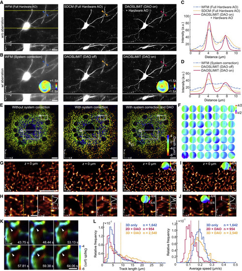
Figure 3. Evaluations of tiled aberration corrections with DAO

(A) Orthogonal MIPs of a 100-μm-thick Thy1-YFP brain slice by SDCM, WFM, and DAOSLIMIT without aberrations. The yellow dashed lines indicate the region for xz projection.

(B) Orthogonal MIPs of the same area after introducing a specific aberration obtained by WFM and DAOSLIMIT with and without DAO. Groundtruth aberration is shown in the inset of WFM result, while estimated aberration by DAO is shown in the DAOSLIMIT result.

(C and D) Cross-section profiles marked by the arrows in (A) and (B), respectively.

(E) Color-coded MIPs of the 3D mitochondrial dynamics by DAOSLIMIT with no corrections, system corrections only, and full DAO corrections.

(F) Estimated average aberrations at different areas in (E).

(G) Reconstructed slice of the region in (E).

(H) Orthogonal MIPs from 2-μm-thick slabs of the region in (E), with cross-section profiles.

(I) Reconstructed slice of (G) with the correction wavefront estimated in (H).

(J) Reconstructed orthogonal MIPs of (H) with the correction wavefront estimated in (G).

(K) Color-coded MIPs of the region in E to show a mitochondrial fusion process.

(L) Histograms of the tracking length and average speed with the same tracking algorithm applied to the 2D video with DAO (n = 954 mitochondria tracked), the 3D video without DAO (n = 1,642 mitochondria tracked), and the 3D video with DAO (n = 2,540 mitochondria tracked). The dashed lines represent the mean values.

Scale bars: 20 μm (A and B), 10 μm (E, G, and I), 2 μm (H and J), and 1 μm (K).

See also Figure S5.

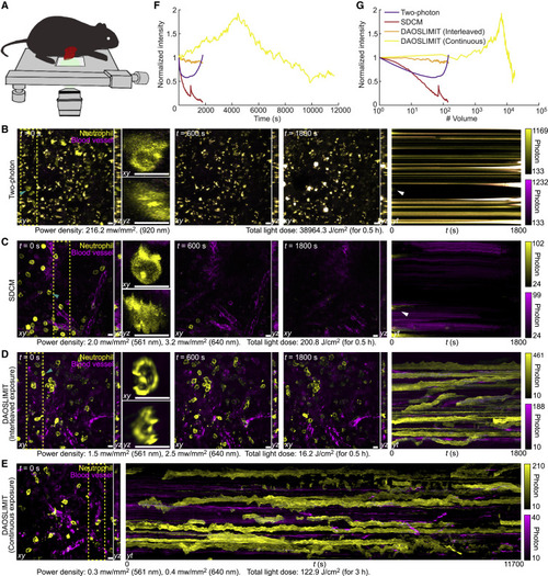
Figure 4. DAOSLIMIT facilitates long-term, high-speed subcellular imaging in mice

(A) Illustrations of the imaging schematic.

(B–D) Orthogonal MIPs (marked by the yellow dashed lines) of the neutrophil (yellow, Ly-6G/Ly-6C) and blood vessels (magenta, WGA) at different time stamps, imaged by high-speed two-photon microscopy (B), SDCM (C), and DAOSLIMIT with interleaved exposure (D). The kymograph with MIP along yt plane shows the bleaching process. Both the power densities during excitation and the total light doses are marked at the bottom. All the methods captured ∼150 two-color volumes.

(E) Orthogonal MIPs and the kymograph obtained by DAOSLIMIT with continuous exposure at 3 volume/s for over 3 h, corresponding to 17,550 two-color volumes.

(F and G) Curves of the normalized average intensity versus time (F) and the number of volumes (G) for the yellow channels. Scale bar, 10 μm.

See also Table S1 and Video S2.

Figure 5. Migrasome dynamics during neutrophil migration in mouse liver (A) MIPs with magnified views illustrating the formation of migrasomes during neutrophil (yellow, Ly-6G/Ly-6C) migration along vessels (magenta, WGA; Video S3, part I). (B) Comparisons between two-photon microscopy, SDCM, and DAOSLIMIT. (C) Migrasome formation with gradually increasing fluorescence (Video S3, part II). (D) Average temporal trace of the newly generated migrasome marked with the red box in (C). (E) 3D migration of one migrasome in a vessel with a temporal-coded trace (Video S4, part I). (F) One migrasome remained attached to the vessel (Video S4, part II). (G) The migrasome generated by one neutrophil was picked up by another neutrophil (Video S4, part III). (H) Division process of a migrasome attached on the vessel (Video S4, part IV). Scale bar, 10 μm. See also Videos S3 and S4.

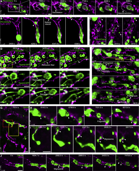
Figure 6. Membrane dynamics during tumor cell migration in zebrafish and mice

(A) MIPs showing the vasodilation process before the tumor cell (MDA-MB-231, green, PH-mCherry) migrated and the vasoconstriction after the tumor cell was washed away by blood flow in zebrafish larvae. The contour profiles of the vessel are marked by dashed lines.

(B) A tumor cell split a large vesicle when trapped in small-bore vessels (magenta, Tg(fli:GFP)) in zebrafish larvae (Video S5, part I).

(C) Various vesicles flowing in the zebrafish vessel (Video S5, part II).

(D and E) Formation of retraction fibers and migrasome-like vesicles during tumor cell (Tspan4-GFP) migration in zebrafish vessels (Video S5, part III).

(F) The tumor cells were pulled back along the retraction fibers against the blood flow in zebrafish larvae (Video S5, part IV). The directions of blood flow and cell movement are labeled by yellow and white dashed arrows, respectively.

(G) Membrane dynamics of injected HeLa cells (green, CM-DiI dye) in the vasculature (magenta, WGA) of a mouse liver (Video S5, part V).

(H) A trapped HeLa cell split a large fragment.

(I) A HeLa cell generated retraction fibers and produced migrasomes during migration.

(J) Another migrasome generation process during the HeLa cell migration in mice (Video S5, part V). Scale bar, 10 μm.

See also Video S5.

Figure 7. 3D calcium dynamics in human cerebral organoids, Drosophila larvae, and zebrafish larvae

(A) Color-coded MIPs of GCaMP6s-labeled human 3D cerebral organoids.

(B) Temporally coded MIPs of the selected area in (A). Different colors correspond to the start time.

(C) Orthogonal MIPs at different time stamps (Video S6, part I).

(D) Temporal traces (ΔF/F₀) of the ROIs labeled in (A).

(E) Color-coded MIPs of Drosophila larval Cho neurons labeled with the jGCaMP7s indicator.

(F) Temporal-coded MIPs for the start time.

(G) Orthogonal MIPs at different time stamps (Video S6, part II).

(H) Temporal traces (ΔF/F₀) of the ROIs labeled in (E). The red arrow indicates the 500-Hz sound stimulus.

(I and J) Orthogonal MIPs of GCaMP6s-labeled zebrafish larva imaged by traditional LFM (I) and DAOSLIMIT (J) (Video S6, part III).

(K) Temporal traces of the same neurons obtained by LFM and DAOSLIMIT marked by arrows in (I) and (J). Scale bars: 10 μm (A–G) and 30 μm (I and J).

See also Video S6.