Figure 2

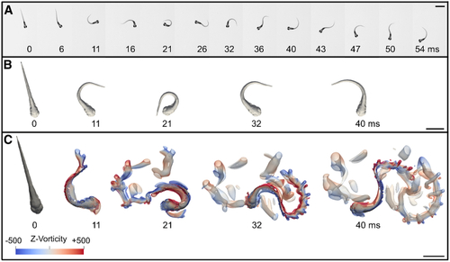
An experiment-driven numerical approach generated a digital reproduction of the zebrafish escape response triggered by an EFP stimulation

(A) Snapshots of an experimental motor response of the first six tail bends/beats recorded at 10,000 frames per second. This escape motor response was a complex behavior composed of three sequential movement forms: a high-amplitude bending of the tail and body (C-bend) (0–11 ms) followed by a high-amplitude counterbend (11–21 ms) and a bout of fast swimming with regular amplitude beats (21–54 ms) to move away from the mimetic predator.

(B) Body movements used as input to the Navier-Stokes solver. From swimming videos (A), image segmentation and Procrustes analysis isolated fish body movements from rotational and translational displacements. The virtual 3D zebrafish was then bent over time to fit with the observed isolated body movements. Resulting 3D snapshots were displayed for the maximal body curvature of the first four tail bend/beat cycles.

(C) Flow generation during escape response numerical simulations. Fluid flow was visualized as the iso-contour of the Q-criterion colored by fluid vorticity in rotations per second (sˆ-1) along the vertical axis (z axis) at the indicated points in time. The complex escape motion (C) was computed from the actual input-based isolated 3D body movement snapshots shown in (B), reproducing the experimental dynamics (A). Aside from the strongest vortex in the fish wake, there were many smaller secondary vortex structures. They may have been caused by the lack of smoothness in the second derivative (acceleration term) of the recorded body movements. The smoothness of the image acquisition could indeed have influenced the simulation since the image acquisition time was about ten times longer than the timestep of the simulation. Panel B shows the fish body movement with translation and rotation subtracted by Procrustes analysis. As a consequence, the yaw angle (heading) was different from that of the real fish swimming in Panel A. Panel C corresponds to the Navier-Stokes solver, which recalculated the translation and rotation motions, explaining why the yaw angles were consistent with those of panel A, but not with those of panel B. On the other hand, the body curvature at each time point remained the same in all three panels. Scale bars: 1 mm.