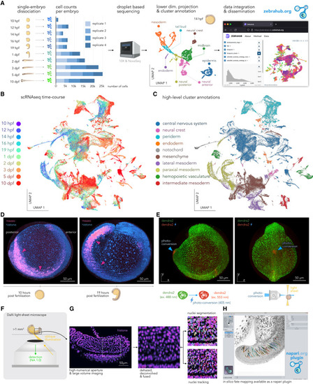
Zebrahub—multimodal zebrafish developmental atlas (A) Zebrahub’s scRNA-seq experimental pipeline for single-zebrafish-embryo single-cell RNA sequencing across developmental stages (dpf, days post-fertilization; hpf, hours post-fertilization). From left to right, we show: first, the number of cells per time point and replicates. Second, an example UMAP for a 14 hpf embryo transcriptome colored by cell type (3,862 cells total). Third, Zebrahub’s web portal allows the exploration of scRNA-seq data online. (B) UMAP representation of the entire dataset of 40 single-embryo transcriptomes colored by developmental stage (120,000 total cells). (C) Same but colored by annotated cell types. (D) Maximum intensity projections of a 12-h light-sheet live imaging of a zebrafish embryo expressing histone-mCherry (cyan) and mezzo-GFP (magenta). Arrows indicate the mezzo-positive cells. (E) Similar imaging but on a transgenic embryo expressing the photoconvertible protein Dendra2. Photoconverted cells are in red (blue arrows). (F) Overview of DaXi, a high-resolution, large field-of-view and multi-view single-objective light-sheet microscope. (G) Computational pipeline for image processing and nuclei tracking applied to images of a histone-mCherry zebrafish embryo acquired with our DaXi microscope (see STAR Methods). (H) Screenshot of the in silico fate-mapping napari plugin available as part of Zebrahub (Methods S1).

Inter-individual transcriptomic variability analysis (A) Sequencing of sibling embryos enables the study of inter-individual gene expression variance. A UMAP of the single-cell data without batch correction (12 hpf, four embryos, 6,699 cells total). Example of normalized expression of gene ybx1 for four embryos (color coded). (B) We used the Kullback-Leibler divergence (KLD) to quantify the pairwise similarity between probability distribution illustrating variant (top, KLD ≫ 0) and invariant (bottom, KLD ≈ 0) gene expression across embryos. (C) Example distributions for embryo-invariant genes (KLD ≈ 0) at 12 hpf: sox11a, notch1a, and dnaja2a. The x axis indicates the log-normalized expression values, and the y axis shows the density (relative number of cells). Heatmaps show all pairwise KLD values. We summarized these heatmaps per gene by the median pairwise KLD (mpKLD, values above the heatmap). (D) Example distributions for embryo-variant genes (KLD ≫ 0) at 12 hpf: ybx1, tma7, and metap2b. (E) Histograms of mpKLD values scores for all cells at 12 hpf. A few examples of high and low mpKLD genes are shown. (F) Distributions of mpKLD values across all genes at 10, 12, 14, 16, 19, and 24 hpf. In (E) and (F), the top and bottom 2% of genes are indicated as colored areas (p values < 10−15 are marked with an asterisk). See also Figure S2 and Data S1.

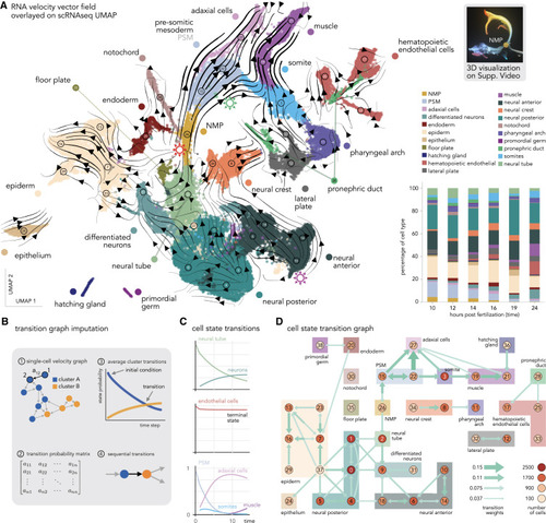
Whole-embryo RNA velocity and derived cell state transition map (A) Projection (UMAP) of zebrafish embryo transcriptomes (early development, 10 to 24 hpf time points), color coded by cell type. Arrow streams correspond to the average RNA velocities of single cells. On the right, stack bar plot of the cell-type proportion over time. (B) Workflow to reconstruct state transitions from RNA velocity graph. (1) Weighted directed graph represents the expected transitions between transcriptional states from single cells. (2) This graph defines a Markov process that can be represented as a matrix. (3) We can then estimate cluster transitions by simulating successive state transitions for groups of cells through the graph. (4) Finally, we summarize cluster-level transitions as a coarse-grained graph. (C) Examples of average transition probabilities for neural tube, endothelial cells, and mesodermal tissue. (D) A coarse-grain graph of cell state transitions shows transitions between all cell states. The width of the arrows is proportional to the transition rates. Colors and numbers correspond to the annotation in (A). Nodes grouped by a bounding box indicate clusters of cells that belong to the same broad cell types; colors correspond to those in (A). Very weak edges should be interpreted with caution, e.g., the connection between germline cells and endoderm might be spurious. See also Video S1C and Data S1.

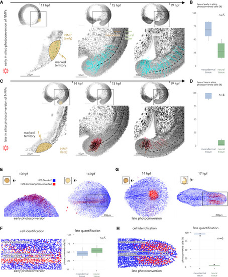
In silico fate mapping of NMPs and in vivo validation via photoconversion and live imaging (A) In silico fate mapping of the pluripotent early NMP territory. Left: selected territory at the initial time point; middle: intermediate time point showing tracks for selected cells; right: final time point. The red star refers to the RNA velocity in Figure 3A. (B) Quantification of early NMP in silico fate mapping with their progeny in the mesodermal (left) and neural (right) fates (n = 5 animals; Data S1). (C) In silico fate mapping of the late presumptive NMP territory. (D) These cells primarily integrate the mesodermal tissue (n = 4 animals; Supp. Fig. 20a). (E) (Right) Photoconversion of the early presumptive NMP territory at ten hpf. (Left) Distribution of the photoconverted cells and their progeny at 14 hpf. (F) (Right) Segmentation and identification of the photoconverted cells in the area selected in (E) left (rectangle). (Left) Distribution of early photoconverted cells and their progeny with mesodermal and neural fates (n = 5 animals). (G) Right: photoconversion of the late NMP territory at 14 hpf. Left: distribution of the photoconverted cells and their progeny cells at 17 hpf. (H) Segmentation and identification of the photoconverted cells in the area selected in (G) right (rectangle). Right: the distribution of the late photoconverted cells and their progeny (n = 6 animals).

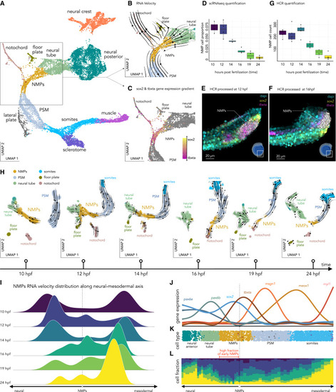
Transcriptional dynamics of NMPs during early development (A) Reprojection (UMAP) of the NMPs and adjacent clusters, color coded by annotated cell types. (B) Zoom in on the NMPs with color-coded cell types and superimposed RNA velocity streamlines. (C) Same projection but with cells color coded by their sox2/tbxta expression ratio; stronger yellow indicates higher sox2 and stronger magenta indicates higher tbxta. (D) Quantifying the proportion of cells in the NMP clusters relative to the total number of cells for each developmental stage. (E) Expression of sox2 (yellow) and tbxta (red) for segmented cells (12 hpf) derived by hybridization chain reaction (HCR). Cells co-expressing sox2 and tbxta, presumptive NMPs, have their boundary in white. (F) Same as (E) but at 16 hpf. (G) Quantification of presumptive NMPs (cells co-expressing sox2 and tbxta) obtained from the HCR image analysis. (H) Velocity trajectories are projected into a time series of aligned UMAPs centered around the NMPs and their adjacent clusters, colored by cell type. (I) Time-resolved quantification of the distribution of RNA velocity for NMPs along the neural-mesodermal axis. These are the normalized distributions of the magnitudes of individual RNA velocity vectors pointing toward either the neural or mesodermal tissues. (J) Pseudotime resolved scaled expression of genes involved in neural development (left axis) and mesodermal development (right axis). (K) Annotated cell-type visualized on the pseudotime axis rooted in the NMPs, recapitulating the neural (left) and the mesodermal (right) developmental transcriptomic trajectories. (L) Cell fraction from different developmental stages visualized along the pseudotime axis.

Zebrahub confirms the existence of early LPM progenitors contributing to pronephron and endothelial cells (A) Reprojection (UMAP) of the lateral plate mesoderm cells and its progeny from Figure 3A UMAP (10–24 hpf). Right: new annotated UMAP and the corresponding velocity. (B) Distribution of the cell time proportion over time. (C) UMAP color coded by time. (D) UMAP plots showing the expression of endothelial/hematopoietic progenitors etv2, tal1, lmo2, the endothelial marker npas4l, the pronephron markers sox17 and pax2a, the erythroid marker hbae3, and the mesothelium marker hand2. (E) In silico photoconversion of the early LPM territory. Left: selected territory at the initial time point. Top right: localization of the cells at the last time points. Bottom right: zoom in on the dashed rectangle (see also Data S1). (F) Transverse schematic section of the zebrafish embryo at 20 hpf. On the UMAPs, the blue arrows indicate the localization of the early progenitors, while the yellow arrows indicate the late progenitors. In the microscopy projection and the transverse section, orange arrows indicate the ISV (intersomitic vessels), while red arrows indicate the pronephron duct.

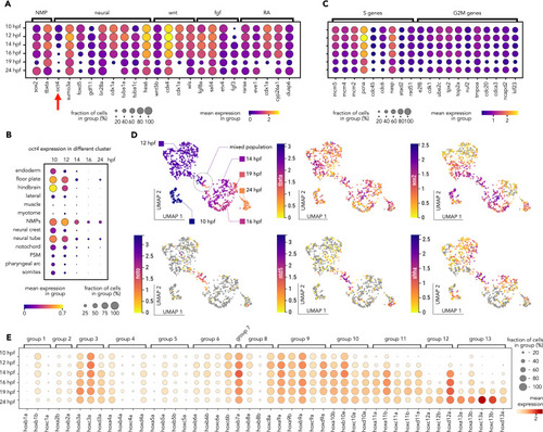
NMP cells’ molecular fingerprints extracted from the scRNA-seq, related to Figure 6 (A) Selection of NMPs enriched genes for signaling pathway important for vertebrates’ axial elongation, showing a peak of expression early during development. (B) Zebrafish oct4 (pou5f3) timeline of spatial expression in the posterior body clusters shows late maintenance of oct4, specifically in the NMP cells. (C) Selection of essential genes for cell cycle enriched in the early NMPs. (D) UMAP embedding of the NMPs cluster in the early integrated UMAP (10, 12, 14, 16, 19, and 24 hpf) color coded by time point (top left). The same embedding is then color coded for the NMP molecular signature genes (sox2 and tbxta) and three important genes for notochord development. (E) A dot plot of the zebrafish hox genes’ expression over time in the NMP clusters shows a collinear activation of the hox pathway.

Distribution of UMIs and detected genes per embryo and Zebrahub parameters versus existing dataset, related to Figure 1 (A) The number of detected UMIs per cell for each embryo. Individual embryos are shown in the x axis sorted by developmental time point (n = 40 embryos, 10 developmental time points). The distribution of UMIs per cell is shown as a boxplot. (B) An equivalent plot for the number of detected genes per cell. (C) Number of cells compared to other scRNA-seq of zebrafish development up to 24 hpf. (D) Number of genes per cell compared to other scRNA-seq of zebrafish development up to 24 hpf. (E) Number of cells compared to other scRNA-seq of zebrafish development after 24 hpf. (F) Number of genes per cell compared to other scRNA-seq of zebrafish development after 24 hpf.

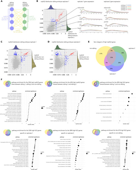
mpKLD for a replicate per sibling and a non-sibling at 24 hpf, related to Figure 2 (A) Schematic representation of the experimental and computational design. (B) The scatter plot with the marginal distribution of mpKLD between replicate 1 and replicate 2. On the right is an example of the mpKLD for four genes with different patterns between replicate 1 and replicate 2. (C) The scatter plot with the marginal distribution of mpKLD between replicate 1 and sibling. (D) The scatter plot with the marginal distribution of mpKLD between replicate 2 and sibling.

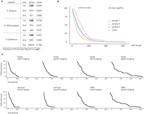
Ultrack is the top-performing algorithm for tracking embryonic development, related to Figure 4 (A) Table summarizing the performance of our tracking solution at the Cell Tracking Challenge for the 3D movie of embryonic development. CZB, CZ Biohub, USA (this paper); KTH, Royal Institute of Technology, Sweden; KIT, Karlsruhe Institute of Technology, Germany; JAN, HHMI Janelia, USA; MPI, Max Planck Institute, Germany; RWTH, Aachen University, Germany. (B) Manual tracking performance of Ultrack reported as track accuracy for three independent samples and all the samples together. In total, we manually curated 427 tracks. (C) Manual tracking performance was reported for different embryonic areas. Overall, better imaging correlates with better tracking.

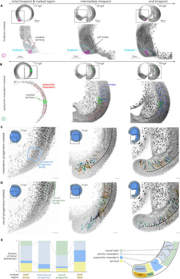
The in silico reconstruction of well-known embryonic lineage and reconstruction of posterior progenitors mapping, related to Figure 4 (A) In silico fate mapping of a population of forebrain cells. Left: selected territory at the initial time point; middle: intermediate time point showing tracks for selected cells; right: final time point. The purple star ∗ refers to the RNA velocity in Figure 3A. (B) In silico fate mapping of the posterior mesodermal progenitors in the presomitic mesoderm. We observe that these cells integrate into the somites that will then generate muscles. (C) In silico fate mapping of the axial mesodermal posterior progenitors. These cells mostly integrate into the mesoderm (74%). (D) In silico fate mapping of the axial neural posterior progenitors. These cells partly integrate the neural tube (46%). (E) Left: the proportion of the clonal distribution after photoconversion of the different progenitor territories: NMPs early (total number of cells = 75), mesodermal progenitors (total number of cells = 81), neural progenitors (total number of cells = 76), NMPs late (total number of cells = 53). Right: a schematic representation of the different axial progenitor territories.

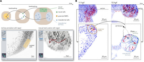
Manual tracking verification of a single NMP, related to Figure 4 (A) Identification of NMPs from territory annotations and backtracking inferred from automatically generated tracking data (top). Screenshot of the napari plugin for in silico fate mapping, showing territory annotation (left) and 3D cell track curation (right). (B) Illustration of a single early NMP (left) dividing into two daughter cells. After cell division, the first daughter.

Tissue morphodynamics constrain the state transition of NMPs during vertebrate body axis elongation, related to Figure 4 (A) Sketch of the dynamic morphoskeleton approach used to identify robust dynamical features from multicellular flows. We focus on repellers—a type of Lagrangian coherent structure locating divergent cell trajectories. We identify repellers by computing the Lagrangian stretching rate ( see Supplemental theory note). (B) Illustration of the time intervals selected to compute the stretching rates, and anatomical annotations of the tail’s territories. NMP, neural and mesodermal tissues. (C) Vector fields representing the cells’ motion during these time intervals, and dashed lines representing the presumptive NMP territory. (D) Lagrangian stretching rate (brighter shades correspond to more stretching, i.e., divergent cell trajectories) and the emergence of repellers in the early NMP presumptive territory. This territory was ascertained by HCR and is outlined by a dashed line.