
- Title
-
Spontaneous and evoked activity patterns diverge over development
- Authors
- Avitan, L., Pujic, Z., Mölter, J., Zhu, S., Sun, B., Goodhill, G.J.
- Source
- Full text @ Elife
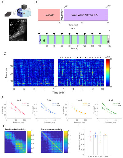
(A) Top: Larvae were embedded in agarose with one eye facing the projected image for two-photon calcium imaging. Bottom: The contralateral optic tectum (in this example 15 dpf) was imaged for 96.6 min. The neuropil (NP) contour of each fish was fitted with an ellipse (dashed line) with the major axis defining the tectal anterior-posterior axis (AP axis). Periventricular layer (PVL), NP, anterior (A) and posterior (P) ends of the tectum are indicated. (B) Experimental protocol. Tectal spontaneous activity (SA) in the dark was recorded after which fish were exposed to light and given 5 min to adjust. We then recorded evoked activity (TEA) in response to 20 trials of the stimulus set consisting of spots at positions 45°, 60°, 75°, 90°, 105°, 120°, 135°, 150°, 165° of the visual field (where 0° was defined as the body axis), presented in an order which maximised spatial separation within a trial. The inter-trial interval was 25 s. (C) Raster plot for an example 15 dpf fish showing concerted neural activity during 8 min of spontaneous activity in the dark and then during three cycles of stimulus presentation (stimulus onset is marked by black triangles). (D) Short-range pairwise correlation coefficients were higher for TEA compared to SA (4 dpf: p=10−4 for up to 50 µm, p=10−3 for 50–100 µm; 5 dpf: p=10−3 for up to 50 µm, p=10−3 for 50–100 µm; 15 dpf: p=10−3 for up to 50 µm, p=10−2 for 50–100 µm). (E) TEA and SA correlation matrices showed structural similarity (example shown is for a 15 dpf fish). Neurons were sorted by their position on the AP axis. (F) Correlation between TEA and SA correlation matrices does not change over development (one-way ANOVA, Bonferroni multiple comparison correction). |
One-way ANOVA, p=0.4. |
( |
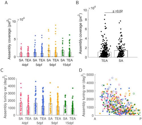
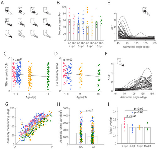
(A) The area covered by the smallest polygon bounding the assembly shows no developmental trend (one-way ANOVA). (B) The area covered by spontaneous activity (SA) assemblies is larger than the area covered by evoked activity (TEA) assemblies (t-test). (C) Assembly tuning variance shows no developmental trend (one-way ANOVA, p=0.66, p=0.62 for SA and TEA respectively). (D) Tuning variance over the anterior-posterior (AP) axis shows a decrease in tuning variance as a function of the assembly centre of mass (CoM). Linear regression EA: p=10−4 for 4 dpf, p=10−4 for 5 dpf, p=10−4 for 9 dpf, p=10−4 for 15 dpf; SA: p=10−2 for 4 dpf, p=10−3 for 5 dpf, p=0.03 for 9 dpf, p=0.09 for 15 dpf. |
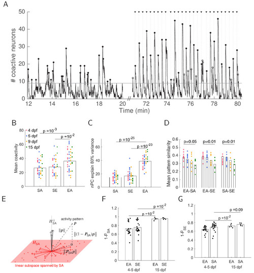
(A) Example showing the number of coactive neurons during 8 min of spontaneous activity in the dark and then during three cycles of stimulus presentation (stimulus onset is marked by black triangles). Significant peaks of coactivity levels (p<0.05, shuffled SA) during SA, EA (black dots), SE (open circles) are marked. (B) There are higher levels of mean coactivity during EA compared to SE and SA (one-way ANOVA, Bonferroni multiple comparison correction). (C) Number of principal components required to explain 80% of the variance (one-way ANOVA, Bonferroni multiple comparison correction) indicates higher dimensionality for evoked responses. In addition to the comparison shown, the dimensionality within the EA epoch increased over development; 4 (dpf) vs. 15 dpf p=0.05, one-way ANOVA, Bonferroni multiple comparison correction. (D) Pattern similarity decreased between all pairs of epochs over development. Similarity was defined as the cosine similarity between the different epochs. (E) Schematic of activity patterns geometry. The patterns of a particular epoch, in this example SA patterns, were collected (red dots), and a linear subspace spanned by these patterns was calculated (HSA, red plane; in reality this is of higher dimension than 2). Given a particular activity pattern 𝒑 (from a different epoch, in this example EA or SE) , 𝑷SA𝒑 is the projection of the pattern onto the subspace HSA. This is the component of the pattern which can be explained by the space HSA, and in the case where the pattern 𝒑 fully resides within HSA, 𝑷SA𝒑=𝒑. Conversely, (𝟙−𝑷SA)𝒑 is the component of the pattern which cannot be explained by the space HSA. It is the projection of the pattern 𝒑 onto the orthogonal complement of the subspace spanned by SA, H1/SA. (F) Projection of EA and SE patterns onto the orthogonal complement subspace spanned by SA patterns indicates that EA and SE patterns are less similar to SA over development. (G) Projection of EA and SA patterns onto the orthogonal complement subspace spanned by SE patterns indicates that EA and SA patterns are less similar to SE over development. |
( |