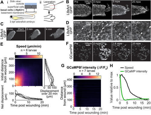
(A) Schematic of (i) bilayered larval zebrafish skin and (ii) laceration technique. (B) Lacerated tailfin over time from a larva 3 days post fertilization (dpf) expressing LifeAct-EGFP in basal cells (TgBAC(∆Np63:Gal4); Tg(UAS:LifeAct-EGFP); Tg(hsp70:myl9-mApple)). mpw: minutes post wounding. (B–F) are all maximum-intensity Z-projections of spinning-disk confocal images. (C) Individual cell from 3 dpf larva expressing LifeAct-EGFP mosaically in basal cells (TgBAC(∆Np63:Gal4) larva injected with UAS:LifeAct-EGFP plasmid at the 1-cell stage). Wound was to the right approximately 1–2 min earlier. (D) Cells in a lacerated tailfin over time from 3 dpf larva expressing LifeAct-EGFP in basal cells (TgBAC(∆Np63:Gal4); Tg(UAS:LifeAct-EGFP); Tg(hsp70:myl9-mApple)), approximately 1–2 min post wounding. Arrowheads: examples of individual actin-rich protrusions are followed over time. (E) Kymograph indicating the speed of basal cells at a given distance from the wound over time (N = 8 larvae). Line graphs show net displacement over space (right) and time (bottom) for each individual larva. See Methods and Figure 1—figure supplement 1 for details of motion tracking analysis. (F) Lacerated tailfin from larva expressing GCaMP6f in basal cells (TgBAC(∆Np63:Gal4) larvae injected with UAS:GCaMP6f-P2A-nls-dTomato plasmid at the 1 cell stage). mpw: minutes post wounding. Due to the large dynamic range in GCaMP intensity, these images were gamma-corrected with a gamma of 0.5 for display purposes. (G) Kymograph of GCaMP6f intensity, normalized by the coexpressed nuclearly localized dTomato intensity, and relative to the normalized intensity pre-wounding (F₀) (N = 7 larvae). (H) Line graph of normalized profiles of the average speed and GCaMP intensity over time, averaged over 300 µm of tissue closest to the wound. To emphasize comparison of the temporal relationship, profiles are rescaled to lie between 0 and 1 (in arbitrary units).

(A) Representative images from timelapse imaging of cellular response to laceration or tail transection. 3 dpf larvae expressing LifeAct-EGFP in basal cells (TgBAC(∆Np63:Gal4); Tg(UAS:LifeAct-EGFP); Tg(hsp70:myl9-mApple)) were anesthetized with Tricaine and wounded by laceration or tail transection (see Methods) and imaged with spinning-disk confocal microscopy. Shown is Z-projections of the LifeAct signal from two representative larvae. (B) Average speed in tissue <300 µm from the wound for laceration or tail transection. Error bars are bootstrapped 95% confidence intervals of the mean. (C) Overview of procedure for tissue motion analysis. 1. Z-projection of LifeAct; myosin light-chain signal is also acquired but not shown. 2. Images of LifeAct are registered using the myosin light-chain signal to remove whole-larva drift not due to cell migration. 3. Thousands of feature points are detected throughout the tissue to use as fiducials for motion tracking from frame to frame (for clarity only 15% of the feature points detected in this frame are shown). 4. Feature points are tracked from frame to frame, reporting motion at different locations in the tissue over time. For clarity 10 randomly selected points are shown. 5. Motion is quantified at different positions in the tissue by averaging the movement of feature points across the tissue. Feature points are binned by their distance from the wound, projected along a line extending from the wound centroid anteriorly through the tail.

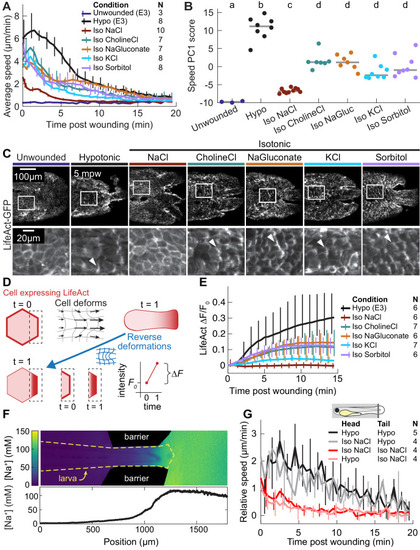
(A) Basal cell speed over time, averaged over 300 µm adjacent to the wound in each larva. 3 dpf larvae expressing LifeAct-EGFP in basal cells (TgBAC(∆Np63:Gal4); Tg(UAS:LifeAct-EGFP); Tg(hsp70:myl9-mApple)) were incubated in E3 (Hypo) or E3 supplemented with 270 mOsmol/l of indicated osmolytes (Iso) and then the tailfin was lacerated and movement analyzed as described in Methods and Figure 1—figure supplement 1. N indicates the number of larvae in each condition. Error bars are bootstrapped 95% confidence intervals of the mean for each condition. (B) Speed trajectories for each larva were analyzed with PCA (see Figure 2—figure supplement 1A–C) and each trajectory’s score along the first principal component is plotted. Gray bars indicate the mean PC1 score for that condition. Letters a-d indicate statistically distinguishable (significantly different) means (p<0.001, one-way fixed-effects Welch’s ANOVA F(6, 19)=130.9, with Games-Howell post-hoc tests). See Table 1 for p-values from post-hoc tests. (C) (Top) Representative tailfins from unwounded larvae or larvae wounded in different media. Images shown from 5 min post wounding. (Bottom) Insets shown below each image. Arrowheads: examples of polarized LifeAct intensity, in the direction of the wound. (D) Schematic of computational procedure for analyzing changes in intensity, after warping image to account for cell/tissue deformation. See Methods for more detail. (E) Relative pixel-wise change in LifeAct intensity over time, averaged over 300 µm adjacent to the wound in each larva. Error bars are bootstrapped 95% confidence intervals of the mean. (F) (Top) Image displaying the device allowing for different media compositions around the tailfin or the rest of the larva. Sodium concentration was calibrated with a sodium-sensitive fluorescent dye. (Bottom) Graph indicates the average sodium concentration along a line across the middle of the image. (G) Relative tissue speed for larvae with different media around their anterior or posterior, as shown in the diagram. To account for residual whole-larva movement due to peristaltic flow, the average tissue speed >300 µm away from the wound was subtracted from the average speed <300 µm away from the wound. Error bars are bootstrapped 95% confidence intervals of the mean.

(A–B) Variation along 1^st (A) and 2^nd (B) principal components of speed trajectories. PC1 captures overall amplitude of the migratory response, while PC2 captures the timing of the peak migratory response. The average trajectory across all conditions is shown in black, and the mean trajectory ±1 standard deviation along the principal component are shown in red and blue, respectively. (C) Percent variance explained by each of the first 10 principal components. (D) Speed trajectories projected onto the space spanned by the first two principal components. Each dot represents the speed trajectory from one larva. (E) Examples of non-rigid deformation approach to measure changes in actin intensity. Shown is a small region of the LifeAct signal in basal cells over time, either the original maximum-intensity projection (original), the image after non-rigid deformation (registered), or the relative change in fluorescence intensity in the registered image (∆F/F₀). Green and magenta arrowhead show particular LifeAct-rich protrusions; filled arrowheads show the original position of the protrusion, while empty arrowheads show the corresponding position of the protrusion in subsequent frames—which differs due to cell and tissue movement. Registration by non-rigid deformation tracks protrusions and warps the image so all changes in intensity of a protrusion occur at the original location of the protrusion in the first frame. Changes in LifeAct intensity in these protrusions are captured in the ∆F/F₀ image at their original position. (F) Average speed trajectories for larvae anesthetized with Tricaine or alpha-bungarotoxin. Data for larvae treated with Tricaine is the same as shown in Figure 2A. Spikes in the alpha-bungarotoxin condition are due to residual larval twitching due to incomplete muscle relaxation. Error bars are bootstrapped 95% confidence intervals of the mean. (G) Two-chamber device schematic. (i) Line drawing used in laser cutting pieces of acrylic to make the mold for the two-chamber device. Gray bar indicates the region that was etched rather than cut, to a depth of approximately 375 µm. (ii) Schematic of the final device made out of PDMS, with holes punched for fluid inlet. Larvae are immobilized in the device as shown with agar around the anterior part of the fish. (iii). Picture of the assembled acrylic mold, with metal bar to create a gap for holding the larvae and for fluid inlets. (iv) Photo of the assembled PDMS device cast from the mold, with inlet tubes added. (v) Photo of the device in a microscope stage insert with inlet and outlet tubes in place. (vi) zoom-in of the device showing the positioning of the inlet and outlet tubes for both chambers to allow independent media exchange in each chamber.

(A) Overview of volume measurement for cell clusters. Representative cluster of cells from three dpf larvae mosaically expressing cytoplasmic mNeonGreen in basal cells (TgBAC(∆Np63:Gal4) embryos injected with UAS:mNeonGreen-P2A-mRuby3-CAAX plasmid at the 1 cell stage). (Left) Z-projection of a representative cell cluster before and 90 s after wounding. (Center) side view at the position indicated by the yellow line. (Right) cell height measured at each pixel. (B) Average volume over time for cell clusters exposed to different media, relative to their volume before wounding. n: number of cell clusters. N: number of larvae. Error bars are 95% bootstrapped confidence intervals of the mean. (C) (Left) Absolute volume measurements for different cell clusters before and 90 s after wounding. *p<0.05, two-tailed t-test on the average paired difference from each larva. See Table 2 for exact p-values and Cohen’s d. (Right) mean paired difference of the measurements shown at left. Distributions are kernel density estimates. (D–E) Average tissue speed (D) and cell cluster volume (E) over time for larvae treated with different concentrations of sodium chloride. 5 and 135 mM speed data are the same as in Figure 2A; 5 and 135 mM volume data are the same as in (B). (F) Average cell cluster volume 90 s after wounding relative to pre-wounding volume, plotted against the average 1^st principal component score for speed trajectories. Error bars are 95% bootstrapped confidence intervals of the mean. Linear regression of the Hypo and three NaCl conditions displayed with a dashed line (r² = 0.95).

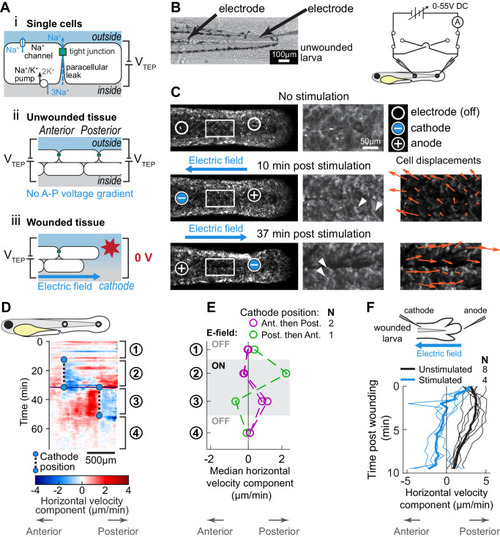
(A) (i) Schematic of the origin of the transepithelial potential (TEP) due to circulating flow of sodium ions. Other ions (such as chloride) may also be transported using energy derived from the sodium-potassium pump, and are not shown here for clarity. (ii) Unwounded tissue does not show an anterior-posterior TEP gradient. (iii) Wounding short-circuits TEP leading to an anterior-posterior TEP gradient and electric field. (B) (Left) Brightfield image of tailfin from 3 dpf larva expressing LifeAct-EGFP in basal cells (TgBAC(∆Np63:Gal4); Tg(UAS:LifeAct-EGFP)), with electrodes inserted under the skin. (Right) Electrical stimulation circuit with variable DC voltage, current measurement, and switches to reverse current polarity in the larva. (C) Z-projections of LifeAct signal from larva shown in (B). (Top) electric field off; (Middle) electric field on with cathode at anterior electrode; (Bottom) electric field reversed with cathode at posterior electrode. Stills are from one continuous timelapse. Insets are shown, and displacement vectors from tissue motion tracking are shown in orange. Arrowheads: examples of polarized LifeAct intensity oriented toward the cathode. (D) Velocity kymograph from a representative timelapse. Color indicates horizontal velocity component from tissue motion tracking analysis. Blue circles and dashed lines indicate the position of the cathode when the electric field was turned on, roughly corresponding to the empty circles on the larva diagram. Numbers 1–4 indicate different phases of the timelapse. 1: electric field off; 2: electric field on, cathode anterior; 3: electric field on, cathode posterior; 4: electric field off. (E) Median horizontal velocity component from three different larva. Tissue velocity was averaged in the region between the two electrodes and then the median velocity during each phase 1–4 (described above) was plotted. For one larva (shown in green) the cathode was initially positioned at the posterior electrode and was then switched to the anterior electrode. (F) Average horizontal velocity component from stimulated or unstimulated larvae. In the stimulated condition, 3 dpf larvae expressing LifeAct-EGFP in basal cells (TgBAC(∆Np63:Gal4); Tg(UAS:LifeAct-EGFP); Tg(hsp70:myl9-mApple)) were impaled with one electrode, with the other electrode positioned immediately posterior to the tailfin. Larvae were then wounded and the electric field turned on, with the cathode positioned at the anterior electrode. Tissue motion between the cathode and the wound was analyzed. Thin lines represent velocity for each larva. Thick lines represent average over larvae. Unstimulated data is the same as in Figure 2A.

(A) Equivalent circuit diagram for the stimulation setup. Electrical resistance comes from the electrodes (measured resistance of ~18.5 MΩ), the resistance to ion flow through the larva itself, and the resistance to flow through the external medium (‘shunt’ pathway of current that does not travel through the larva). Shunt and larval resistance are not directly measured. See Methods for discussion of these different parameters. (B) Estimate of current density in the larva. (Left) Maximum-intensity projection of a larva expressing hsp70:myl9-mApple, which labels all the cells. (Upper right) Cross section through the trunk suggests that the dimensions of the larva in the trunk can be approximated as ~80×130 µm. (Lower right) The larval cross-section is simplified as a rectangle for estimation purposes. Three different possible regions through which current could flow are depicted, and the current density resulting from a 1µA current flowing through each of these regions is shown below each region.