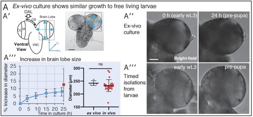
(A) Diagram of the chamber and sample preparation for long-term time-lapse imaging on an inverted microscope (see Materials and methods). (B) 24 h, confocal 3D time-lapse imaging of a developing larval brain lobe (inset, top left, shows orientation and region of the brain imaged) labelled with Jupiter::GFP and Histone::RFP, and registered over time to account for movement. Arrowheads indicate NBs (magenta) and progeny (cyan), enlarged in the top right insets; a dashed white line indicates the boundary to the optic lobe. (C′) A typical individual dividing NB from a confocal time-lapse image sequence of the brain lobe. The NB is outlined (dashed white line) and indicated with a magenta arrowhead, the progeny (GMC) is indicated by a cyan arrowhead. (C′′) Plot of NB division rate for cultured L3 brains shows that division rate of NBs does not significantly decrease over at least 22 h under imaging conditions (n = 3 brains, not significant (ns), p=0.87, one-way ANOVA), calculated from measured cell cycle lengths. (D′) Typical GMC division in an intact larval brain. The first row of panels shows production of a GMC (cyan arrowhead) by the dividing NB (magenta arrowhead, dashed white outline). Second row of panels, GMCs are displaced over the next 6 to 8 h by subsequent NB divisions, the path of displacement is indicated by the dashed yellow arrow. The last two panels (10 to 18 min) show the division of a GMC (green arrowhead, progeny yellow arrowheads). (D′′) Plot showing the rate of GMC division in the ex vivo brain does not change with time in culture (n = 4 brains, ns, p=0.34, one-way ANOVA), calculated from the number of GMC division events in 4 h. Error bars on plots are standard deviation. Scale bars (B) 50 µm; (C), (D) 10 µm.

Related to Figure 1 (A′) Left panel: diagrammatic overview of the Drosophila wandering third instar larval stage (wL3) brain highlighting the dorso-anterior-lateral region of the central brain which contains neural stem cells of the type I NB lineage. CB central brain; OL optic lobe; M medulla; VNC ventral nerve chord; DAL dorsal anterior lateral region. Right panel: an ex vivo brain imaged in bright field, the blue arrows indicate measurements taken of brain lobe diameter to assess growth in culture. (A′′) Analysis of the increase in brain lobe size in culture compared to in vivo. The left plot shows ex vivo cultured brain lobe diameter increase for Jupiter::GFP; Histone::RFP L3 brains over 24 h (blue trace, n = 3) under wide-field fluorescence imaging conditions. The single red datapoint shows average lobe diameter (n = 13) for freshly isolated brains from free living larvae at the end of wL3, corresponding to the stage expected for 24 h culture. The right hand plot directly compares brain lobe diameter for 24 h cultured and freshly isolated brains from free living larvae at the end of wL3 (ns, Mann-Whitney test, ex-vivo n = 4; in-vivo n = 25). (A′′′ and A′′′′), bright field images at two time-points during culture and examples of freshly dissected free living larvae at corresponding developmental stages, respectively. Scale bars 50 µm.

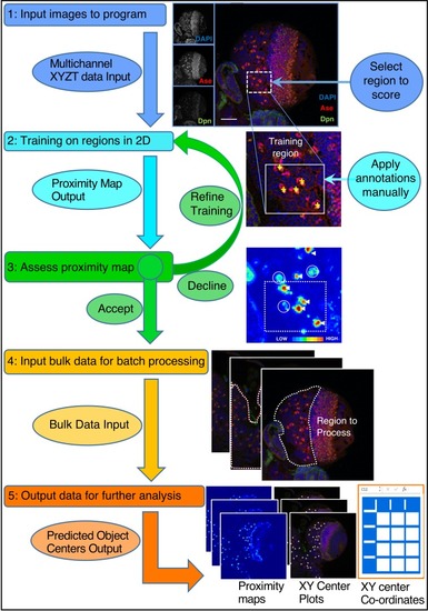
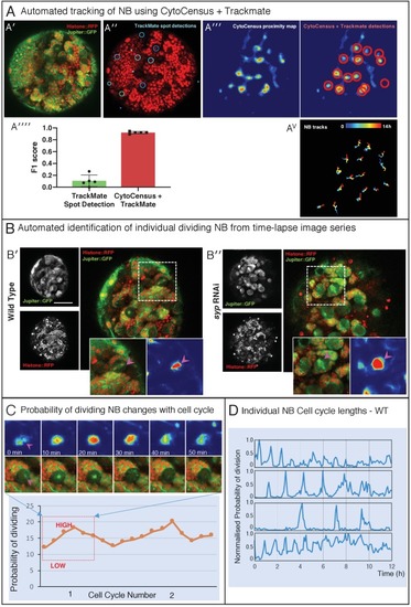
Refer to the Main Text and Materials and methods for details. Training is performed by single click annotation (yellow crosses) within a user-defined region of interest (ROI, white dashed square) to identify the cell class of interest. The resultant proximity map for cell class identification (~probability score for object centres) is evaluated manually to assess the success of training (white arrows indicate good detections and circles indicate where more training may be required). A successful identification regime (Model) is saved and may be used to batch process multiple image data sets. Multiple outputs are produced including a list of the co-ordinates of identified cells. Multiple identification regimes can be sequentially applied to identify multiple cell classes from a single data set.

Related to Figure 2 (A) Snapshot of the user interface for ‘Training ‘(above) and ‘Evaluate’ batch processing (below), with the user defined settings enlarged to the right (for more details see the ‘User Manual’ associated with the Supplemental material). (B) Output results summary for automated detection of a cell class: count; probability map, predicted centres overlay; XY co-ordinates for predicted centres.

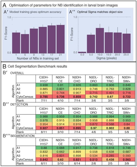
(A) Performance in identifying NBs from 3D confocal image data of a live brain labelled with Jupiter::GFP, Histone::RFP. (A′) Ground Truth manual identification of NB centres. A′′ to ′′′′) Output images comparing NB identification by Ilastik, Fiji-Weka and CytoCensus, white overlay. (Av) Plot comparing object centre detection by TrackMate spot detection, RACE, Fiji-Weka, Ilastik Pixel Classification and CytoCensus (error bars are standard deviation). CytoCensus achieves a significantly better F1-score than Ilastik (p=0.01, n = 3) and FIJI (p=0.005, n = 3). (one-way RM-ANOVA with post hoc t-tests) (B) Comparison of algorithm performance for a 3D neutral challenge data set (B′, see Materials and methods). (B′′, B′′′) Output images comparing object centre determination by Ilastik Pixel Classification and CytoCensus. Segmentation results are shown as green outlines, object centre determination is show as a cyan point. (B′′′′) Plot comparing object centre determination accuracy for the 3D neutral challenge dataset (error bars are standard deviation; p<0.001, Welch’s t-test, n = 25). Scale bars (B) 20 µm; (A′) 50 µm.

Related to Figure 3. Examples of automated detection of (A) Type-I NBs and (B) GMCs, respectively, from a 3D multichannel image set for a fixed WT larval brain labelled with DAPI, anti-Ase and anti-Dpn. In both cases, training was performed by single click annotation within a user defined region of interest (ROI, dashed lines in A′′ and B′′) to identify the cell class of interest. The resultant ‘proximity’ maps (A′ and B′) and corresponding cell class identifications (e.g. A′′ and B′′) were evaluated manually to assess the success of training. The zoomed regions (corresponding to the dashed white boxes) show examples of correct identification (cyan arrowheads) and false negative (magenta arrowheads) of NB in A′V) and GMC’s in B′V). (C) Manual identification of cell classes from generic labels: fixed Jupiter::GFP, Histone::RFP labelled brain (C′), immunolabelled for Dpn and Pros (C′′) to permit unequivocal identification of NB and their progeny. (D) Validation of CytoCensus identification of NB and progeny from generic cytological makers. (D′) Cell centre predictions are shown from CytoCensus analysis of the dataset from (C′) with generic markers. (D′′) Corresponding identifications of NB and progeny based upon Dpn and Pros markers. (D′′′) Plot showing that identification based upon Jupiter::GFP, Histone::RFP labelling alone effectively identifies NB and progeny compared to identification from Dpn and Pros labels: 96% ± 4 NB identification (n = 12, three repeats) and 92% ± 2 progeny identification (n = 189, three repeats). Scale bars (A′′) and (B′′) 50 µm; (C′) and (D′) 20 µm.

Related to Figure 3. (A’ A’) The F1-score (see Supplemental Information) was plotted for different levels of training from annotation of a single NB cell, up to annotations of 21 individual NBs. As training examples are added, results improve but rapidly approach maximum with little training (A′′) F1-score for varying sizes of sigma (radius of cell detection in pixels). Performance is optimal at sigma = 10, which is slightly smaller than the radius of a NB. (B′) Cell Segmentation Benchmark overall performance (mean of Detection and Segmentation scores) (B′′) Cell Segmentation Benchmark Detection performance (B′′′) Cell Segmentation Benchmark Segmentation performance. Colours indicate ranking (red = worst, green = best).

Related to Figure 4. (A) Comparison of brain lobe diameter (A’) Brightfield images of WT, syp and syp RNAi (A’’) Average of two manual measurements/lobe (as per Figure 1—figure supplement 1A). Lobe diameter is increased in syp (WT vs syp, p<0.0001, t-test with Tukey correction, n = 12), and syp RNAi (WT vs syp RNAi p=0.0022, t-test with Tukey correction, n = 5) (B) Immunofluorescence analysis shows absence of Syp expression in syp RNAi, and syp mutant brains. Brains are labelled with DAPI, anti-Syp and Jupiter::GFP. Scale bar 25 µm.

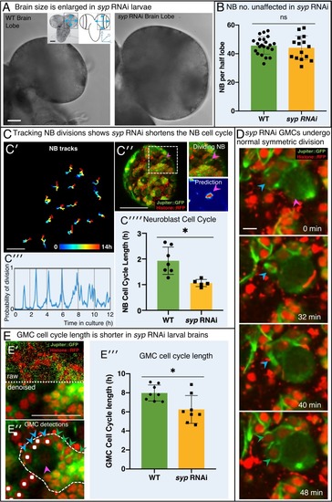
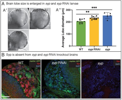
(A) Brightfield images of freshly isolated brains from third instar WT (OregonR) and syp RNAi larvae, respectively. Inserts in (A) show the region of the brain imaged and the measurements taken to compare brain size. (B) Chart comparing NB numbers showing that syp RNAi knockdown does not have a significant effect on NB number/brain (ns, p=0.77, t-test, WT n = 22; RNAi n = 15). NB were identified by Dpn labelling and the average count for a comparable volume of a single optic lobe CB region is shown. (C) Automated identification of NB division using CytoCensus: (C′) Tracking of NB centres, based on CytoCensus detections, over 14 h; (C′′) raw image showing single timepoint from live, 3D time-lapse, confocal imaging (insert = single dividing NB, showing CytoCensus prediction of a dividing NB); (C′′′) graph of division of a single tracked NB over 14 h; (C′′′′) average NB (6–9 NB/brain) cell cycle length is reduced in syp RNAi knockdown brains (p=0.004, Welch’s t-test, WT n = 7, syp RNAi n = 5 brains); (D) Sequence of confocal images from a typical 3D time-lapse movie showing that in syp RNAi brains, GMCs divide normally to produce two equal sized progeny that do not divide further. (E) Semi-automated analysis of GMC division by CytoCensus shows that GMC cell cycle length is reduced in syp RNAi brains. (E′) Single image plane taken from a 3D time-lapse, confocal image data set (imaged at one Z-stack/2 min). showing raw image data (top) and denoised (bottom). (E′′) CytoCensus GMC detections (cyan) with a single NB (magenta), and NB niche (dotted white line), shows GMCs are detected but neurons (green) are not. (E′′′) Plot of GMC cell cycle length, which is decreased in syp RNAi brains compared to WT (p=0.01, Welch’s t-test, n = 8 GMCs from three brains). Scale bars in (A) 50 µm; (C′) 20 µm; (C′′) 50 µm; (D) 5 µm; (E) 25 µm

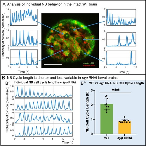
(A) Using the proximity map output of CytoCensus, individual NBs can be followed through their cell cycle. Arrows: Individual NB locations, and the corresponding proximity map output plotted over time for that NB. (B) Comparison of WT and syp RNAi NB: (B′) analysis of cell cycle over time for individual NBs from a syp RNAi brain; (B′′) comparison of cell cycle lengths for individual NB in a single WT vs syp RNAi brain (p=0.002, F-test, n = 9 NB). Scale bar 40 µm

Related to Figure 5. (A) Tracking of NB with TrackMate and CytoCensus (A′-A′′) Raw image, and histone-based detections of NB (cyan circles) from TrackMate (A′′′) CytoCensus NB proximity map, and corresponding TrackMate detections (red circles) (A′′′′) Graph of F1-score of raw TrackMate detections and CytoCensus proximity map with TrackMate detections (A^V) NB tracks that span the whole 14 hmovie from CytoCensus + TrackMate (B) Automated identification of individual dividing NB for time-lapse series using the probability density map output of CytoCensus. (B′-B′′) Show WT and syp RNAi brains, with inset highlighting an individual dividing NB (marked with anti-Ase, anti-Dpn and DAPI) and their corresponding proximity maps. Scale bar is 50 µm. (C) Change in proximity score (probability of division) plotted over time for an individual WT NB undergoing division: upper panels are the confocal images and corresponding proximity maps; lower panel is a plot of probability covering two cell cycles, the region corresponding to the images above is highlighted. (D) Series of plots showing different NB over time, and the changes in the probability of dividing (B) as they progress through the cell cycle.

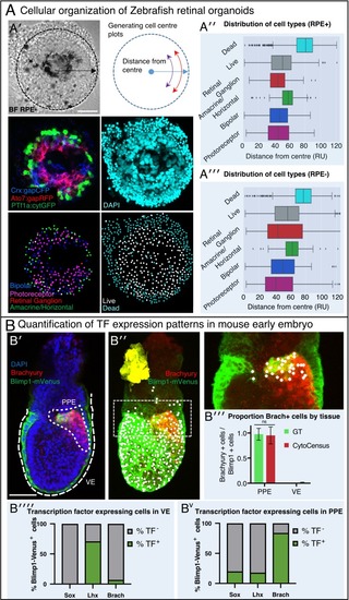
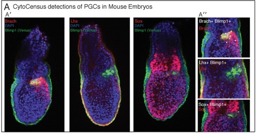
(A) Automated analysis of Zebrafish retinal organoids at the single-cell level. Raw data from Eldred et al. (2017). (A′) Top: brightfield image and diagram indicating the location of cells was defined as displacement from the organoid center. Middle: Cell fate marker expression (Crx:gapCFP; Ato7:gapRFP; PTf1a:cytGFP) and DAPI. Bottom: Cell centre identification by CytoCensus for the different cell types as defined by the labelling profiles (Bipolar, Photoreceptor, Retinal Ganglion, Amacrine/Horizontal, Live/Dead). (A′′-A′′′) Radial distribution of the different cell types determined from cell centre identifications by CytoCensus; the effects on organoid organisation of the presence (A′′) or absence (A′′′) of retinal pigment epithelium (RPE) cells is examined (ns, one-way ANOVA). RU = Radial Units, normalised to a radius of 100 (see Materials and methods) (B) Automated quantification of TF expressing cells in a fixed early streak stage mouse embryo (e6.5) labelled for transcription factors, Blimp1-mVenus and DAPI. (B′) A medial confocal section showing Brachyury in the primitive streak in the proximal posterior epiblast (PPE) and visceral endoderm (VE, highlighted cortical tracing). (B′′) Cortical image of the same mouse embryo overlaid with total cell centre predictions by CytoCensus of Brachyury positive cells; insert to the right is a zoomed in image of the highlighted rectangle showing only cell centre predictions in a single medial plane. (B′′′) Comparison of CytoCensus and manual Ground Truth (GT) measurements of the proportion of Brachyury positive cells from 2D planes in the VE and PPE (ns, t-test, n = 3). (B′′′′-Bv) Proportion of transcription factor positive cells (TF) in, using CytoCensus measurements in 3D according to tissue regions (PPE and VE) defined in (B′). Scale bars 25 µm in (A); 100 µm in (B′).

Related to Figure 6. (A′) Image plane through centre of each embryo used for quantification illustrating the different distributions of TF⁺ cells. Images marker with DAPI, Blimp1-Venus and antibody against (Brach, Lhx, Sox) (A′′) TF⁺ (Brach, Lhx, Sox) PGC detections in the proximal posterior epiblast (PPE), quantified in Figure 6B.