Processing steps for the generation of a LoG scale-space maximum intensity projection used for 2D seed detection.

Original image (A), LoG filtered image with σ = 5 and σ = 8 (B, C), LoG scale-space maximum intensity projection with σ min = 5, σ max = 8 and σ step = 1 (D) and the detected seeds plotted on the original image (E).

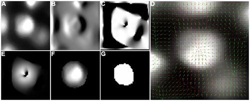
Processing steps that are performed in parallel for each detected seed point.

Cropped raw image (A), Gaussian smoothed left-right derivative image (B), dot product of the normalized gradient with the seed normal (C), raw image with smoothed gradient and normal vector field overlay (D), weighted version of the previously calculated dot product (E), resulting intensity image (F) and the final segmentation result (G).

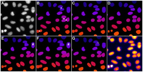
Comparison of the segmentation quality achieved by the investigated algorithms on 2D benchmark images from the Broad Bioimage Benchmark Collection (BBBC006v1).

Original image (A), adaptive thresholding using Otsu’s method [23] (B), Otsu’s method combined with watershed-based blob splitting [23], [30] (C), geodesic active contours [31] (D), gradient vector flow tracking [16] (E), graph-cuts segmentation [17] (F), TWANG segmentation (G) and a false colored original image (H). The symbols indicate segmentation errors for nuclei that are either split (#), merged (+), missing (o) or spurious (~).

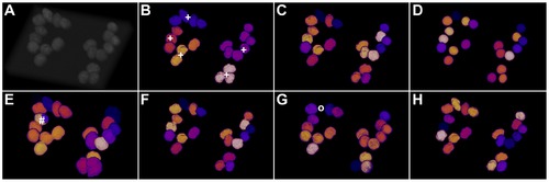
Comparison of the segmentation quality achieved by the investigated algorithms on simulated 3D benchmark images by Svoboda et al. (HL60 cell line, low SNR, 75% clustering probability)[35].

Simulated original image (A), adaptive thresholding using Otsu’s method [23] (B), Otsu’s method combined with watershed-based blob splitting [23], [30] (C), geodesic active contours [31] (D), gradient vector flow tracking [16] (E), graph-cuts segmentation [17] (F), TWANG segmentation (G) and the simulated ground truth image (H). The symbols indicate segmentation errors for nuclei that are either split (#), merged (+), missing (o) or spurious (~).

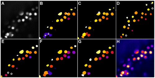
Comparison of the segmentation quality achieved by the investigated algorithms on a 3D image of labeled nuclei of a zebrafish embryo acquired using DSLM.

The panels show the maximum intensity projection of 3 neighbouring z-slices. Original image (A), adaptive thresholding using Otsu’s method [23] (B), Otsu’s method combined with watershed-based blob splitting [23], [30] (C), geodesic active contours [31] (D), gradient vector flow tracking [16] (E), graph-cuts segmentation [17] (F), TWANG segmentation (G) and a false colored original image (H). The symbols indicate segmentation errors for nuclei that are either split (#), merged (+), missing (o) or spurious (~).

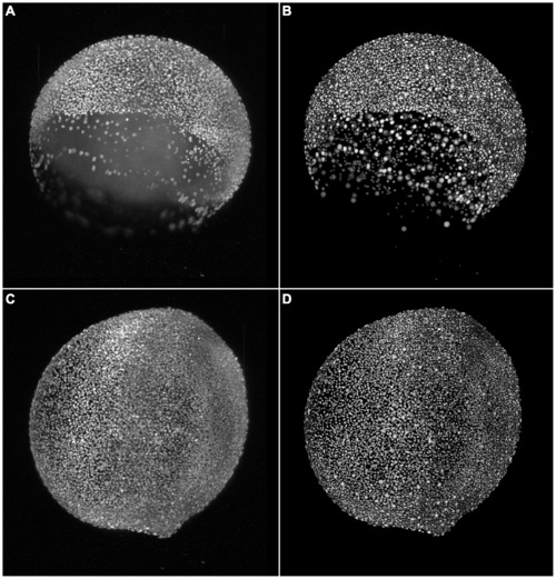
Results of the TWANG segmentation pipeline applied on two images of a developing zebrafish embryo.

The images were captured at the 7≈8000 cells (A,B) and at the 11 hpf stage with ≈12000 cells (C,D), respectively. The panels show maximum intensity projections of the raw images (A,C) and the resulting segmentation using our TWANG segmentation pipeline (B,D). Each 3D image stack has a file size of ~5GB and comprises 2560×2160×500 voxels with a dynamic range of 16 bits. Processing one image stack takes approximately 10-20 minutes on a common desktop machine, depending on the developmental stage of the embryo. Typical experiments may be comprised of up to 2000 z-stacks (~10TB) for the spatio-temporal analysis of a single embryo.