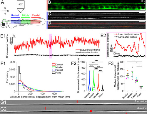
The Reissner fiber under tension exhibits spontaneously dynamic behavior over the dorsoventral axis in the central canal.

(A) Spinning disk confocal microscopy setup using a 40X objective with 3 dpf Tg(sspo:sspo-GFP) zebrafish larvae for live imaging. Schema of zebrafish larva designates rostral (blue), middle (green) and caudal (red) sections, corresponding to somites 1–10, 11–20, 21–30, respectively. (B) Immunohistochemistry with anti-GFP antibodies in 3 dpf Tg(sspo:sspo-GFP) larva after fixation shows RF with the floor plate (FP) visible within the caudal somites of the spinal cord. (C) Live imaging snapshot of RF in the rostral somites of a 3 dpf Tg(sspo:sspo-GFP) paralyzed, living larva (top) and larva after fixation (bottom). (D) Example tracking of continuous motion of RF through the development of a script to model its movements in the dorsoventral axis. (E1) Example trace of the change in dorsoventral position of RF in one paralyzed, living larva (red) and another euthanized larva after fixation (black) over a 25 s timelapse acquired at 40 Hz. Data was discretized in 2 μm bins along the rostrocaudal axis before plotting. (E2) Zoomed-in display of the highlighted area marked on E1, showing a trace of the dorsoventral position of RF over 1 s for both the paralyzed, living larva and the euthanized larva after fixation, respectively, with circles indicating the sampling points. (F1) Displacement in the dorsoventral axis for paralyzed larvae (N=4 rostral, 4 middle, 4 caudal recordings) is significantly larger than that of fixed (N=4 recordings) larvae on average median ± standard deviation provided hereafter: in paralyzed living larvae = 74 nm ± 68 nm versus in fixed larvae = 32 nm ± 39 nm; unpaired two-tailed t-test: p < 10^-4. The displacement was calculated from data that was discretized in 2 μm bins along the rostrocaudal axis. (F2) Dorsoventral displacement of RF is significantly different among rostral, middle and caudal segments of paralyzed larvae (on average median ± standard deviation in rostral somites = 100 nm ± 103 nm versus in middle somites = 125 nm ± 108 nm versus in caudal somites = 70 nm ± 68 nm versus in fixed larvae = 32 nm ± 39 nm; Tukey’s HSD Test for multiple comparisons: p < 10^-4). (F3) Median dorsoventral displacement of RF from the mean position per fish, with each color representing a different fish (on average mean of median dorsoventral displacement ± standard deviation in rostral somites = 107 nm ± 25 nm versus in middle somites = 117 nm ± 37 nm versus in caudal somites = 72 nm ± 12 nm versus in fixed larvae = 28 nm ± 7 nm; Tukey’s HSD Test for multiple comparisons: p < 0.05). (G1–G2) A principal component analysis was computed on one image sequence of one fish (with each image corresponding to one observation) to understand the most significant movements of the fiber. The G1 component corresponds to a dorsoventral translation (the fiber borders are black on the ventral side, white on the dorsal side) and G2 to a small local rotation around a point (in red). These two components account respectively for 21.9% (G1) and 3.4% (G2) of the total temporal variability in the video. * p < 0.05, **** p < 10^-4. Scale bar is 10 μm (B, C, D) and 20 μm (G1, G2).

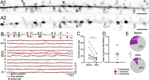
The Reissner fiber enhances spontaneous calcium activity in ventral CSF-cNs.

(A1) Time-series standard deviation projection in the sagittal plane from two-photon laser scanning microscope showing the signal from the Reissner fiber and CSF-cNs in the central canal of 3 dpf Tg(sspo:sspo-GFP;pkd2l1:tagRFP;pkd2l1:GCaMP5G) zebrafish larva before RF photoablation. (A2) Time-series standard deviation projection in the sagittal plane from two-photon laser scanning microscope showing the signal from CSF-cNs after RF ablation performed by spiral scanning photoablation with an infrared pulsed laser tuned at 800 nm over 0.5 μm on RF (see Materials and methods). (B) ROI selection for ventral CSF-cNs to analyze activity before and after RF photoablation within the same cells (top). Example calcium activity traces normalized to baseline for each of the ROIs before (red) and after (black) RF photoablation over 75 s imaged at 3.45 Hz (see Materials and methods). (C) Percentage of active ventral CSF-cNs (active is defined as having at least 1 calcium transient during the recording) before and after RF photoablation (N=109 cells total from 8 fish from two independent clutches; mean percent active before ablation = 27.72% ± 6.34% versus mean percent active after ablation = 10.59% ± 3.1%; paired two-tailed t-test: p < 0.05). (D) The ratio of active ventral CSF-cNs after RF photoablation to those active before RF photoablation, illustrating on average, a fraction (on average ± SEM: 45% ± 14%) of active ventral CSF-cNs before photoablation remain active after RF photoablation. The purple lines on the graph represent the mean and the error bars indicate the SEM. (E) Pie charts illustrating the number of events per ventral CSF-cN before and after RF photoablation (mean number of events in active cells before RF photoablation = 0.94 events/min versus mean number of events in active cells after RF photoablation = 0.87 events/min; paired two-tailed t-test: p < 0.005). * p < 0.05, **p < 0.005. Scale bar is 20 μm (A1, A2), 10 μm (B).

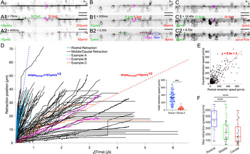
Reissner fiber photoablation reveals different modes of relaxation under tension

(A) Frame-by-frame instantaneous speed calculations for the rostral and caudal ends of the cut RF during retraction after photoablation by UV-pulsed laser in 3 dpf triple transgenic Tg(sspo:sspo-GFP;pkd2l1:tagRFP;pkd2l1:GCaMP5G) paralyzed larvae. Pink spiral indicates the site of RF ablation. Instantaneous speeds of the fiber for both rostral and caudal ends were calculated using the change in position of the fiber between two consecutive frames, divided by the exposure time (25 ms) and converted to μm/s. (A1, A2) specifically depict an example of a fiber in the ‘rigid case’, where the fiber retracts straight on both ends without distortion. (B) Instantaneous speed calculations for both rostral and caudal ends of a cut fiber in the ‘relaxed case’, where there is distortion of the fiber (B1 left cut end, B2 right cut end) due to no more tension on one or both ends of the fiber. By analogy with the dynamics of DNA molecules, one can refer to the completely relaxed portion of the fiber as the ‘flower’, while the remaining taut portion of the fiber would be the ‘stem’. (C) Instantaneous speed calculations for both rostral and caudal ends of a cut fiber that remains stuck in the central canal, remaining in the field of view for about 25 s. (D) Retraction position plotted across the square root of time for all fish (N=74 fish from 7 independent clutches), color-coded to illustrate the examples in (A–C), and indicating if a flower was seen in the 38 s-long recordings along the rostrocaudal axis. D×Δ⁢LL is provided by the slopes of the two dotted lines (blue and red), indicating a fast retraction or a slow retraction of the rostral and caudal ends of the cut fiber in the central canal. Inset: initial retraction speed (the distance the cut fiber retracted in between 50 ms and 75 ms after photoablation, after UV laser artifacts) is larger in the fibers classified under the fast retraction group than those in the slow retraction group. (E) Rostral and caudal ends of the fiber in cases with and without flowers plotted against each other, demonstrating that rostral and caudal end dynamics generally tend to mirror each other (N=74 fish). (F) Maximum retraction speed for rostral and caudal ends of the cut RF classified using the schema in Figure 1A, grouping the ablations that occurred in the rostral somites (N=9 fish), middle somites (N=34 fish), and caudal somites (N=34 fish). Mean for ablation in rostral somites = 448 μm/s ± 168 μm/s versus in middle somites = 253 μm/s ± 166 μm/s versus in caudal somites = 211 μm/s ± 165 μm/s; Tukey’s HSD Test for multiple comparisons: p < 10^-4. ****p < 10^-4. Scale bar is 10 μm (A, B,C).

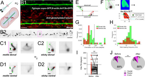
The Reissner fiber interacts with beating cilia protruding in the central canal. (A) Schematic illustrating motile cilia (white) lining the walls of the central canal beside CSF-cNs (red) with RF (green) bathing in the spinal cord of a zebrafish larva. (B1) Z-stack projection in the sagittal plane showing the immunostaining against GFP and glutamylated tubulin in a Tg(sspo:sspo-GFP;-ß-actin:Arl13b-GFP) larva fixed at 3 dpf revealing respectively RF and cilia labeled by the ß-actin promoter (both in green here) and motile cilia (red). Rostral to the left, ventral displayed on the bottom. (B2) Single optical section in the sagittal plane showing RF surrounded by cilia protruding in the central canal in 3 dpf Tg(sspo:sspo-GFP;ß-actin:Arl13b-GFP) paralyzed larva out of the streaming video acquired at 40 Hz using spinning disk confocal microscopy setup equipped with a 40X objective. (C1) Right: example single optical section of a dorsal motile cilium from the highlighted box in (B1). Dark green arrow indicates RF. Light green and red dots indicate the base and tip of the cilium, respectively. Left: average projection over 25 s of the dorsal cilium brushing against RF. (C2) Right: example single optical section of a dorsal motile cilium whose tip tends to stick to RF. Left: average projection over 25 s of the dorsal cilium. (D1) Right: example single optical section of a ventral motile cilium whose tip tends to brush against RF. Left: average projection over 25 s of the ventral cilium. (D2) Right: example single optical section of a ventral motile cilium whose tip tends to stick to RF. Left: average projection over 25 s of the ventral cilium. (E) Schematic illustrating the geometric calculation of ciliary orientation versus the dorsoventral axis. (F) Representative analysis process for the dorsal cilium in (C2). A mask was first drawn over a single cilium to calculate the frequency and orientation in a specific region of interest (left). A temporal mean of that region (middle) was then used to calculate the orientation of the cilium in respect to the dorsoventral axis (right; see also Materials and methods). (G1) Distribution of the orientation in respect to the dorsoventral axis of dorsal mean ± standard deviation provided hereafter: (64.8° ± 44.4°; N=49 cilia across 8 fish) and ventral (43.9° ± 35.8°; N=27 cilia across 9 fish) motile cilia. (G2) Distribution of main ciliary beating frequency for dorsal (mean ± standard deviation provided hereafter: 11.8 Hz ± 2.7 Hz; N=49 cilia) and ventral (11.6 Hz ± 2.8 Hz; N=27 cilia) motile cilia. (H) The orientation of motile cilia in the central canal was not significantly different after RF photoablation (mean ± standard deviation provided hereafter: 55.1° ± 39.3°) from that before RF photoablation (57.4° ± 42.5°), illustrating that cilia orientation is, on average, not significantly affected by RF photoablation (N=76 cilia from 9 fish; paired two-tailed t-test: p > 0.3). (J) Overall rostrocaudal polarity of motile cilia remained similar before and after RF photoablation, with about 90% of motile cilia polarized toward the caudal end of the fish, and the remaining 10% either polarized toward the dorsal end of the fish or beating in the Z axis (N=76 cilia from 9 fish; paired two-tailed t-test: p > 0.3). ns = not significant. Scale bar is 10 μm (B1, B2) and 2 μm (C1, C2, D1, D2).

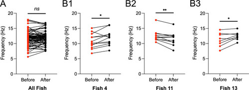
Changes in the main ciliary beating frequency varied from fish to fish in response to RF photoablation.

(A) The main beating frequencies of dorsal and ventral motile cilia after RF photoablation (mean ± standard deviation provided hereafter: 11.9 Hz ± 2.0 Hz) compared to those before RF photoablation (11.7 Hz ± 2.4 Hz), illustrating that cilia main beating frequency was on average not significantly affected by RF photoablation (N=76 cilia from 9 fish; paired two-tailed t-test: p > 0.3). (B1–B3) Select examples from (A), depicting fish whose response to RF photoablation significantly changed the main ciliary beating frequencies but in different ways. B1 and B3 illustrate an increase in main ciliary beating frequency after RF photoablation (B1: mean ± standard deviation provided hereafter: 11.9 Hz ± 2.5 Hz; B3: 12.5 Hz ± 1.4 Hz) from that before RF photoablation (B1: 10.9 Hz ± 2.5 Hz; N=12 cilia; paired two-tailed t-test: p < 0.05; B3: 11.3 Hz ± 2.3 Hz; N=8 cilia; paired two-tailed t-test: p < 0.05). B2 illustrates a decrease in main ciliary beating frequency after RF photoablation (11.6 Hz ± 2.2 Hz) from that before RF photoablation (12.6 Hz ± 1.9 Hz; N=11 cilia; paired two-tailed t-test: p < 0.01). * p < 0.05, ** p < 0.01.

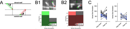
Motile cilia position profile differs with Reissner fiber dorsoventral oscillation position.

(A) Schematic illustrating the geometric calculation of ciliary orientation versus the dorsoventral axis. (B1) Top: two k-means clusters of a single optical section in the sagittal plane demonstrating a dorsal motile cilium brushing along the RF in the central canal in a 3 dpf Tg(sspo:sspo-GFP;β-actin:Arl13b-GFP) paralyzed larva out of the streaming video acquired at 40 Hz using spinning disk confocal microscopy setup equipped with a 40X objective. Dark green arrow indicates the RF. Light green and red dots indicate the base and tip of the cilium, respectively. Rostral to the left, ventral displayed on the bottom. Bottom: frequency distributions of the two dorsal cilium clusters (found by performing k-means clustering using two clusters for RF position in the dorsoventral axis) plotted according to the two RF clusters corresponding to oscillatory up and down movements. The cilium and RF positions were found dependent (Fisher’s exact test: p < 0.05). (B2) Top: two k-means clusters of a single optical section in the sagittal plane demonstrating a ventral motile cilium brushing along the RF for the same paralyzed larva in (A1). Bottom: frequency distributions of the two k-means ventral cilium clusters plotted according to the RF position (k-means clusters corresponding to up or down RF movement in the dorsoventral axis). The cilium and RF positions were found dependent (Fisher’s exact test: p < 0.01). (C) Left: orientation of the two k-means clusters (average) for dorsal cilia plotted as a function of the RF position in the dorsoventral axis (two k-means clusters representing up and down movements), whose histograms (as in B1) were statistically significant (blue; N=7 dorsal cilia across 5 fish) and those that were not statistically significant (black; N=15 dorsal cilia across 5 fish). Right: orientation of the two k-means clusters (average) for ventral cilia plotted as a function of the RF position in the dorsoventral axis (two k-means clusters representing up and down movements of the fiber), whose histograms (as in B2) were statistically significant (blue; N=4 ventral cilia across 5 fish) and those that were not statistically significant (black; N=9 ventral cilia across 5 fish). * p < 0.05, ** p < 0.01. Scale bar is 2 μm (B1, B2).

Example cilia analysis process.

(A) Example of a single optical section showing a dorsal cilium from Figure 4C2. Dark green arrow indicates the RF. Light green and red dots indicate the base and tip of the cilium, respectively. (B) A mask drawn over the single cilium to calculate only the frequency and orientation in a specific region of interest. (C) The raw fluorescence trace of the inside of the mask over 25 s video (left) and zoomed in over 1 s (right), corresponding to the highlighted area on the left panel, was used to detect peaks and estimate the ciliary beating frequency by counting the number of oscillations per second. (D) The temporal mean of the time series was calculated to see a temporally smoothed overview of the video. (E) Standard deviation projection over 25 s before temporal smoothing. (F) A principal component analysis was performed to grasp which movements of the cilium could explain the most variability, which appeared in PC1 (left) and PC2 (right). (G) Ciliary orientation calculation. Left: window to calculate the orientation manually. Green dot represents the predetermined cilium center from the polyfit function in MATLAB. Black and red dots represent the manual inputs for the base and tip of the cilium, respectively. Right: The value for the manual calculation of orientation was compared to the orientation output of the two MATLAB functions and the one determined to best explain the data (in this case, a tilt of 52.7°) was kept for further analyses. Scale bar is 2 μm (A).