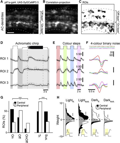
Recording AC functions in vivo (A–C) Example scan of syGCaMP3.5-expressing AC dendrites within the IPL, showing the scan average (A); a projection of local response correlation, indicating regions of high activity (B); and the correspondingly placed ROI map (C). Scale bar, 5 μm. (D–F) Example regions of interest (ROIs, cf. C), with mean trial averages (black) superimposed on individual repeats (gray) to the three light stimuli tested: an achromatic chirp stimulus (D), four spectrally distinct steps of light from dark (red, green, blue, UV, as indicated; STAR Methods) (E), and a spectral noise stimulus used to establish linear filters (kernels) at the same four wavelengths (F). (G) Distribution of ROIs from the central (black, n = 927 ROIs, 10 scans, 6 fish) and peripheral retina (white, n = 816 ROIs, 10 scans, 6 fish) by polarity (On/Off/On-Off) and kinetics (transient/sustained). Chi-square test, p < 0.001 for both datasets. (H) Distribution of kinetic component weights (STAR Methods; cf. Figure S1B) of central and peripheral ROIs. Wilcoxon rank-sum test, p < 0.001 for all four datasets.

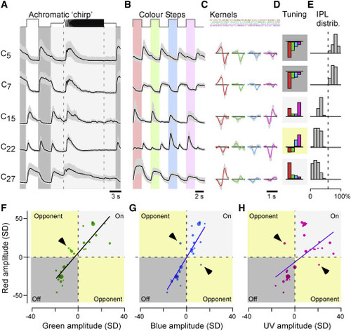
ACs are kinetically diverse but spectrally simple (A–E) Example cluster means ± SD in response to the white chirp (A) and color-step stimuli (B), spectral kernels (C) corresponding to mean kernel amplitudes (D), and each cluster’s distribution across the IPL (E). Shadings in (D) annotate cluster polarity (dark, Off; light, On; yellow, color opponent). (F–H) Relationship of each clusters’ kernel amplitudes (n = 27 clusters) in red (y axis) plotted against the corresponding amplitudes in green (F), blue (G), and UV (H). Note that most points scatter across the two non-opponent quadrants of the plots, with exceptions highlighted by arrowheads. Dot size indicates the number of ROIs in a cluster. Non-weighted line fits are superimposed for illustration.

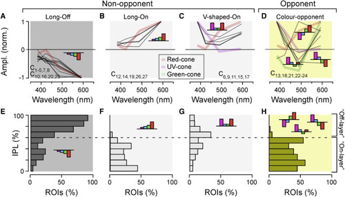
ACs are kinetically diverse but spectrally simple (A–D) Spectral tuning functions of all AC clusters (gray lines), allocated to one of four groups as shown: long-wavelength-biased Off (A) and On (B), V-shaped On (C), and color opponent (D). Plotted behind the AC spectral tunings are reduced tuning functions of selected cones (cf. Figures S5B and S5C) to illustrate qualitative spectral matches between cones and AC clusters. Clusters contributing to each group are listed in each panel. (E–H) Corresponding IPL distribution of AC ROIs allocated to each of the four spectral groups, as indicated.

Effects of AC blockage on BCs (A and B) Example scan field (A) and ROI mask (B) of a typical scan from BC terminals expressing SyjGCaMP8m,44,45 with approximate IPL boundaries and On/Off layer separation indicated. Scale bar, 5 μm. (C–E) Example ROIs from (A) and (B) as indicated, responding to the white chirp (C) and color steps (D), alongside mean spectral kernels recovered from 4-color noise stimulation (E). (F–H) As (C–E), respectively, but for three different example terminals that were recorded after pharmacological injections of GABAzine, TPMPA, and strychnine to block inhibitory inputs from ACs. Note that responses are generally larger and more transient compared with control conditions, but diverse spectral opponencies persist. Scale bars: 5 SD (C, D, F, and G), 50 SD (E), and 20 SD (H).

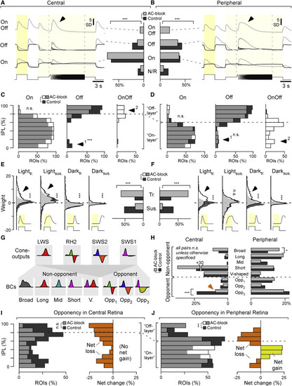
ACs differentially modulate grayscale processing in BCs across the eye (A and B) Bar plots: distribution of BC ROIs recorded in the central (A) and peripheral retina (B) by response polarity (non-responsive, On, Off, On-Off) before (control, dark gray) and after blocking inhibitory inputs (AC block, light gray), as indicated (chi-square tests for the bar plots, p < 0.001 for both datasets), and the corresponding mean response waveform to the white chirp stimulus (cf. Figure 4C) of all terminals in a given category. Arrowheads highlight distinct temporal dynamics during temporal flicker across the regions. Central: n = 1,492 ROIs under the control condition and 1,566 ROIs under the AC block condition from 13 scans in 13 fishes; peripheral: n = 1,526 ROIs under the control condition and 1,639 ROIs under the AC block condition from 13 scans in 13 fishes. (C and D) Distribution of On, Off, and On-Off BC terminals across the IPL, as indicated, with control data shown in dark gray and AC block data superimposed semi-transparently in white, so that overlapping bars appear in light gray. Note that the On/Off boundary differs between the central (C) and peripheral retina (D; see also Bartel et al.,18 Zimmermann et al.,19 and Zhou et al.33). Arrowheads highlight key differences between central and peripheral histogram pairs. Two-sample Kolmogorov-Smirnov test; central: On, p = 0.77; Off, p < 0.001; peripheral: On, p = 0.30; Off, p = 0.11. Because of the absence of data points under control conditions, no statistical tests were used to test changes for On-Off distributions. (E and F), Distribution of kinetic component weights used to fit BCs’ white step responses (cf. Figure S1B; STAR Methods) across the datasets and conditions as indicated (vertical histograms) and distribution into overall transient and sustained response types (bar plots). Arrowheads highlight the major differences across control and AC block conditions in each case. Wilcoxon rank-sum test for the distribution plots, p = 0.93 for the peripheral lightsus group, p < 0.001 for all other groups; chi-square test for the bar plots, p < 0.001 for both datasets. (G) Illustration of how cone input could build the different spectral response types in BCs. Insets indicate approximate spectral tuning functions (amplitude y versus wavelength x). The top row shows the four cones,7 and the bottom row shows BCs,18,19 divided into five non-opponent and three opponent categories. (H) Percentages of ROIs per spectral category (cf. G) based on BC kernels (cf. Figure 4E) for central (left) and peripheral datasets (right). Note that the distribution across spectral categories differs strongly by retinal region, but within a region, most spectral categories are approximately stable between control (dark gray) and AC block conditions (light gray). The main exception to this observation is indicated by the arrow. Wilcoxon rank-sum tests, central: p > 0.05 for the first 7 groups, p < 0.001 for “Opp3” group; peripheral: p = 0.015 for the “Broad” group, p > 0.05 for all others. (I and J) Left: IPL distributions (I, central retina; J, peripheral retina) of all ROIs classed as color opponent during the control condition (dark gray) and following AC block (white, so that their overlay is light gray). Right: difference between control and AC block in each case, with net loss of opponency shown in orange and net gain in yellow. The full datasets leading to the summaries in (H–J) are shown in Figures S7B–S7E. Two-sample Kolmogorov-Smirnov test for changes in IPL distributions of opponent terminals; central, p = 0.39; peripheral, p < 0.001.

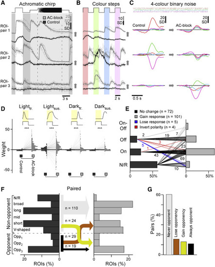
Paired recordings (A–C) Example ROI pairs as indicated in Figures S8A–S8D, illustrating frequently observed effects of AC block on single terminals when probed with the same set of stimuli used to classify all ACs (Figure 1) and BCs (Figure 4). Chirp and color-step traces (E and F) are vertically offset between the two conditions for clarity. (D) As Figures 5E and 5F but here for paired data (n = 182 pairs, from 13 scans, 13 fishes); pairwise weight distributions for the four kinetic components under the control (left) and AC block condition (right), as indicated. (E) Paired BCs automatically sorted by polarity under control (left) and AC block conditions (right). Lines represent the pairs, with numbers of BCs indicated. Chi-square test, p < 0.001. (F) As Figure 5H, allocation of BCs into spectral groups, here shown for a paired dataset, which allowed connecting spectral groups under the control condition (left) and following AC block (right). For simplicity, connections are collapsed into those where there is no change in color opponency (gray, black), where color opponency is lost upon AC block (orange), and where opponency is gained (yellow), with numbers of BC pairs corresponding to each connection indicated. Note that non-responsive terminals are added as one extra non-opponent category, which resulted from the generally lower signal-to-noise ratio in SyGCaMP3.5 recordings compared with the previously used SyjGCaMP8m. (G) Summary of changes to color opponency as shown in (F).

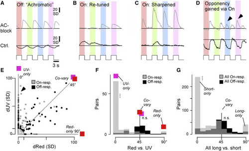
Selective spectral modulation of the On pathway (A–D) Selected example BC color-step responses (trial averages) during the control condition (bottom) and following AC block (top, paired data), illustrating a range of “typical” results. Generally, changes in Off responses tended to be similar across all tested wavelengths (A). In contrast, changes in On responses tended to be more spectrally diverse and often effected a change in overall spectral tuning (B and C), including in spectral opponency (D). Arrowheads in (D) highlight wavelength-specific switches in the On channel that led to a change in color opponency. (E–G) Co-variation of absolute response amplitudes changes (in SD) after AC blockage, compared across different pairs of wavelengths (paired data). (E) shows an individual scatterplot for red versus UV. On and Off responses are plotted separately, as indicated. Correspondingly, an angular histogram (F) was computed from this scatterplot, where 45° indicates co-variation, while peaks around 0° and 90° indicate that one of the two compared wavelength responses changes independently of the other. Data points with an Euclidean distance of less than 10 from the origin were excluded from further analysis (shaded area in E). (F) shows the individual red-UV comparison, while (G) shows the sum of all six possible color combinations (cf. Figure S10). Note that Off responses tended to co-vary (peak at 45°), while On responses exhibited a more diverse distribution, which included peaks at 0°, 45°, and 90°. Wilcoxon signed-rank test for a given color combination; tests were performed between On or Off angular distributions and 45°; all On (G): p < 0.001, all Off (G): p = 0.32; red On (F): p < 0.001 (red versus UV), Off: p = 0.24 (red versus UV).