
- Title
-
Non-telecentric two-photon microscopy for 3D random access mesoscale imaging
- Authors
- Janiak, F.K., Bartel, P., Bale, M.R., Yoshimatsu, T., Komulainen, E., Zhou, M., Staras, K., Prieto-Godino, L.L., Euler, T., Maravall, M., Baden, T.
- Source
- Full text @ Nat. Commun.
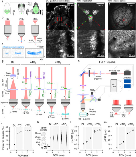
Non-telecentric beam optics in 2-photon microscopy.
a Drosophila (left), larval zebrafish (centre) and adult mouse schematics (right) with central nervous system highlighted (green) to illustrate size differences. Insets next to the mouse for size-comparison on the same scale. b Optical configurations of standard diffraction limited (DL, left) 2P setup with parallel laser beam entering objective’s back aperture. Right, non-telecentric (nTC, middle, right) configurations use a diverging laser beam instead. As a result, the field of view and focal distance are expanded, and the point spread function (PSF) elongates. These effects scale with the angle of divergence (compare nTC1 and nTC2). c Typical neuronal somata in species shown in (a), as interrogated by 2P setups shown in (b), respectively. d In vivo 7 dpf larval zebrafish (HuC:GCaMP6f) imaged with a Sutter-MOM DL setup at full field of view (top) and when zoomed in to reveal individual neuronal somata (bottom) as indicated. e same zebrafish as (d), next to two further zebrafish imaged using nTC2 configuration at maximal field of view (top). Zooming in to the same area as in (d, bottom) reveals cellular detail (e, bottom). f In vivo adult mouse cranial window over somatosensory cortex imaged with nTC2 maximal field of view (top) and when zoomed in as indicated (bottom). g Left: Optical configuration of a standard DL setup with collimation system consisting of a scan lens and a tube lens to set-up an infinity collimated laser beam at the objective’s back aperture. Effective refractive power and relative distances of lenses indicated. The intermediary focal point (IFP) is behind the scan lens (arrowhead). Middle: nTC1 configuration replaces the scan lens with two plano-convex lenses (L1,2). The relative position of L2 to the tube lens defines the position of the IFP, which is now further along the laser path. As a result, the field of view can be expanded to between 1.2 and 1.8 mm. Right: nTC2 configuration using a single plano-convex lens (L3) allows FOV expansion to 2.5–3.5 mm. h complete nTC setup, including an ETL positioned in front of the scan mirrors for rapid axial-scanning. PMTs, Photomultipliers. i FOV expansion under nTC combines two effects: Increased focal distance (left) and reduced numerical aperture (N.A., right), which together yield a larger effective focal plane and enlarged PSF. j Power at sample measured for all configurations, expressed as a percentage of the power that reaches the scanning mirrors. k point spread functions (PSFs) measured for all configurations, with size of typical neuronal somata of different species indicated. All scale-bars 10 µm. l, m, lateral (l) and axial (m) spread of the PSFs quantified. Errors in mean ± s.d., n = 20 experimentally independent samples per measurement. Data leading to j, l, m in Source data file. |
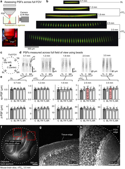
Spatial resolution over the full field of view.
a Schematic (top) and photograph (bottom) of the setup used to directly film excitation volumes. IR, infrared. b effective scan-planes directly visualised as indicated in (a) for all optical configurations as indicated, in each case with scan-points spaced to facilitate inspection of individual PSFs. c–e PSF measurements using fluorescent beads (cf. Fig. 1m) across the full FOV for all optical configurations as indicated in (c). Shown are exemplary scan profiles (pairs of xz and yz projections) from (d) and (e) quantification of full width half maxima (FWHM) In lateral (xy) and axial dimensions (z). For statistical evaluation we compared each “lateral” PSF estimates to the respective centre estimates using 1-way ANOVA. No significant differences were detected, except in two top-right (TR) xy values for nTC2 conditions, as indicated. These small differences are likely explained by slightly imperfect laser centring. Error bars in mean ± s.d., n = 20 experimentally independent samples per measurement. TL, top left, TR, top right, BL, bottom left, BR, bottom right. f–h, example scan under nTC2 3.5 mm configuration of a mouse brain slice labelled with SMI31 for phosphorylated Neurofilament-H (NFH). Full usable FOV (f) and two zoomed in regions (g, h) as indicated in (f), without moving the objective, to illustrate image quality at the FOV edges (f–h, 1024 × 1024 px, 0.49 Hz). Data leading to e in Source data file. |
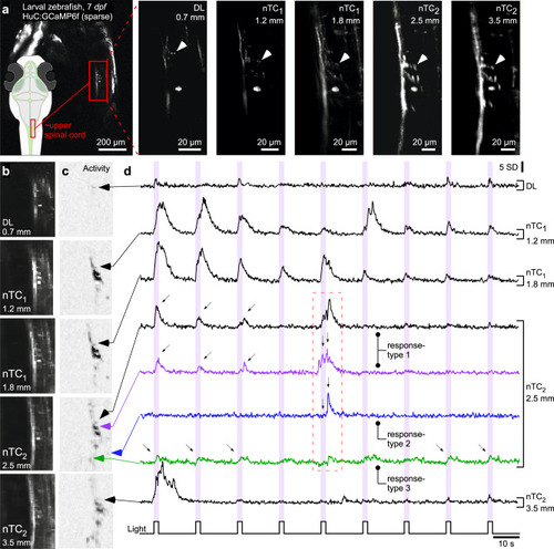
In vivo calcium imaging across different optical configurations.
a The same set of neurons of the 7 dpf larval zebrafish upper spinal cord (HuC:GCaMP6f, random sparse expression, see overview scan and schematic on the left) was imaged in all optical configurations as indicated at 512 × 512 px (1 Hz). Arrowheads highlight the same synaptic structures in each scan. b–d 64 × 64 px (7.81 Hz) activity scan from fields of view shown in (a) for all five configurations during presentation of full-field flashes of UV-light which stochastic elicited activity in these imaged neural structures. In each case the average scan projection (b) and neighbour-correlation based activity projection (c) are shown (hereafter referred to as “activity-correlation”). Darker shadings, equalised for visibility, denotes increased local activity (for details, see ref. 70). Black traces in (d) show time-traces for the same structure in all cases. For the nTC2 2.5 mm FOV condition, time-traces from different neural structures are extracted to illustrate different responses in different structures. All activity traces in this and the following figures are shown in z-scores relative to their own baseline (hence y-scale in s.d.). We choose this metric over dF/F as it emphasises detectability of events rather than the relative change from the indicator’s baseline fluorescence, which differs between biosensors. |

Rapid remote focussing.
a, b, Scan-profiles with the electrically tunable lens (ETL) “flat” (zero input current, lowest profile) and engaged to achieved axially elevated scan planes at +300 and +600 µm (middle, upper profiles, respectively) in nTC1 (a) and nTC2 (b) configuration, as indicated. Associated size-changes in the effective full field of view were generally <5% (compare top and bottom planes). In each case, axial-shifts required <25% unidirectional peak current on the ETL which in turn facilitated rapid ETL-settling times: c, d, Schematic (c) and measured (d) axial jumps and settling time: the ETL was programmed to iteratively focus up and down by 150 µm at each end of two long (5 ms) scan lines, as indicated. This enabled a direct read-out of ETL settling at each line-onset (oscillations in d). For the 150 µm jumps shown, oscillations decayed below detectability within 2–3 ms. For corresponding readouts of the ETL-position signal, see Fig. S3. |
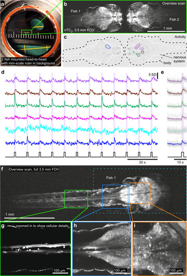
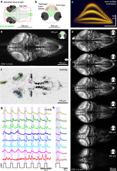
Mesoscale imaging of zebrafish larvae.
a Photograph of two 9 dpf zebrafish larvae mounted head-to-head in a microscope chamber with mm-scale ruler in background. b The same 2 fish (HuC:GCaMP6f) as in (a) imaged under 2-photon with nTC2 3.5 mm FOV configuration, at 512 × 128 px (3.91 Hz). c, d Activity-correlation (cf. Fig. 3c) of the scan in (b) during presentation of full-field flashes of ultraviolet (UV)-light, with hand-selected exemplary ROIs, extracted time-traces (d) and light-stimulus-aligned averages (e). f–i The same fish as shown on the left in (b, fish 1), now shown at full 3.5 mm field of view (f, 512 × 128 px, 3.91 Hz) and increased spatial resolution scans of regions as indicated to reveal cellular detail (g–i, 1024 × 1024 px, 0.49 Hz). RGC, retinal ganglion cell. |
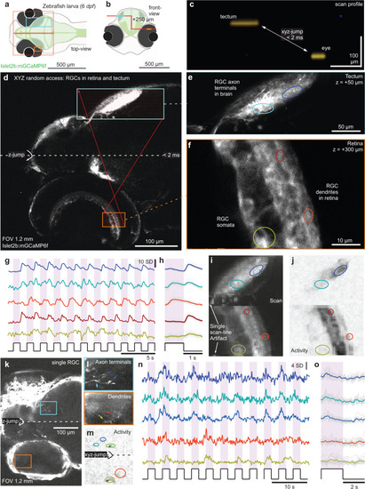
3D random access scanning of the zebrafish eye and brain.
a, b Schematic of zebrafish larva from top (a) and front (b) with scan configurations indicated. c direct x-z visualisation of the scan-profile used in the below. d nTC1 1024 × 1024 px scan across an Islet2b:mGCaMP6f 6 dpf larval zebrafish eye and brain. At the centre of the scan, the axial focus is shifted upwards such that the axonal processes of retinal ganglion cells (RGCs) in the tectum (top) and their somata and dendritic processes in the eye (bottom) can be quasi-simultaneously captured. e, f, 1024 × 1024 px split-plane random access jump between tectum (e) and eye (f) and g–j 2 times 64 × 128 px (15.6 Hz) random access scan of the same scan regions with raw (g) and event-averaged (h) fluorescence traces, mean image (i) and activity-correlation (j, cf. Fig. 3c). The stimulus was a series of full-field broadband flashes of light as indicated. k–o as (d–j), with individual RGCs transiently expressing GCaMP6f under the same promoter. |
2P plane-bending to image the in vivo larval zebrafish brain.
a–c Schematic of HuC:GCaMP6f larval zebrafish brain viewed from top (a) and front (b) with scan planes indicated, and (c) example-scan-profiles. d nTC1 512 × 1024 scans of a 6 dpf zebrafish brain with different plane curvatures, with peak axial displacement at scan centre as indicated. At curvatures ~100–150 µm peak displacement the scan approximately traverses the surface of the tectum. e–h Mean (e), activity-correlation (f, cf. Fig. 3c) and fluorescence traces (g, raw and h, event-triggered mean) from a 170 × 340 px scan (5.88 Hz) of the 100 µm peak displacement configuration (image 3 in (d)). The fish was presented with full-field and spectrally broad (~360–650 nm) series of light-flashes. See also Fig. S4. |
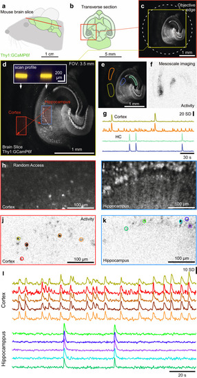
Mesoscale and random-access imaging in mouse brain slice.
a, b Schematic of brain (a) and transverse section (b) of a Thy1:GCaMP6f mouse. c, d 1024 × 1024 px nTC2 example scan of slice through cortex and hippocampus at maximal FOV (c) and nTC2 zoom in (d) as indicated. Red arrows indicate rapid transitions between scan regions, with the inset showing scan-profiles. The slice was bathed in an epileptogenic (high K+, zero Mg2+) solution to elicit seizures. e–g Mean of 256 × 256 px scan (3.91 Hz) of (d) with regions of interest (ROIs) indicated (e), activity-correlation projection (Methods) indicating regions within the scan showing regions of activity computed as mean correlation of each pixel’s activity over time to all its neighbours (for details, see ref. 70) (f) and z-normalised fluorescence traces (g). h–l, 2 times 128 × 256 px (3.91 Hz) random access scan of two regions as indicated in (d) allows quasi-simultaneous imaging of the cortex (h) and hippocampus (i) at increased spatial resolution, with activity-correlation (j, k, cf. Fig. 3c) and fluorescence traces (l) extracted as in (j, k). |
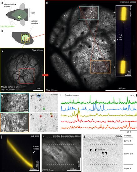
Mesoscale random-access imaging of mouse cortex in vivo.
a,b Schematic of Thy1:GCamP6f mouse brain in vivo (a) with cranial window over the somatosensory cortex (b). c, d 1024 × 1024 px nTC2 (c) and nTC1 (d) images as indicated. Red arrows indicate rapid transitions between scan regions, with the inset indicating the scan-profile. e–i 2 times 128 × 256 px (3.91 Hz) random access scan as indicated in (d) with mean-projection (e, f), activity-correlation (g, h, cf. Fig. 3c) and fluorescence traces (i), taken from the ROIs as indicated in (g, h). j–l nTC1 128 × 128 px xyz-tilted plane (7.82 Hz) traversing through cortical layers 1–4 at ~45° relative to vertical (such that the x-image dimension corresponds to the x-mirror, while the y-dimension in the image represents simultaneous and matched y- and z-movement, with mean image (k) and activity-correlation (i, cf. Fig. 3c). The scan was taken under nTC2 3.5 mm FOV configuration and zoomed in to the central ~0.6 mm. |
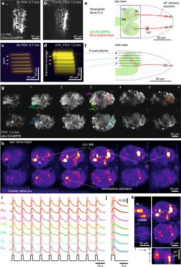
Multi-plane imaging and optogenetics for functional circuit mapping.
a, b, DL (a) and nTC1 (b) 1024 × 1024 px scans of the ventral nerve cord of a 3rd instar (L3) VGlut:GCamP6f Drosophila larva. c–f Scan-profiles taken in DL (c) and nTC1 (d) across 6 planes spaced ~15 µm apart. e, f Schematic of first instar (L1) elav:GCamP6s; Ocro:CsChrimson Drosophila larva from top (e) and side (f), with CsChrimson (red) and GCaMP6s (green) expression pattern and scan-planes indicated. g–k optogenetic circuit mapping of olfactory processing centres across the larval brain. Six scan planes (170 × 340 px each) were taken at 0.98 Hz/plane (i.e. volume rate) during the presentation of 587 nm light flashes (2 s) to activate CsChrimson in olfactory sensory neurons (OSNs). Brain anatomy (g) and false-colour coded fluorescence difference image (h 1–2 s after flash onset minus 1–2 s prior to flash onset), with fluorescence activity traces (i raw and j event triggered average). For a zoom-in on the antennal lobe in a different specimen, see also Fig. S5. k data from (h) summarised: top right: max-projection through the brain, with left and bottom showing transverse max-projections across the same data-stack. VNC, ventral nerve cord. AL, antennal lobe, L(H)/M(B), Lateral horn/Mushroom body, CL, Contralateral (antennal) lobe. |