
- Title
-
Microscale Neuronal Activity Collectively Drives Chaotic and Inflexible Dynamics at the Macroscale in Seizures
- Authors
- Burrows, D., Diana, G., Pimpel, B., Moeller, F., Richardson, M.P., Bassett, D.S., Meyer, M.P., Rosch, R.E.
- Source
- Full text @ J. Neurosci.
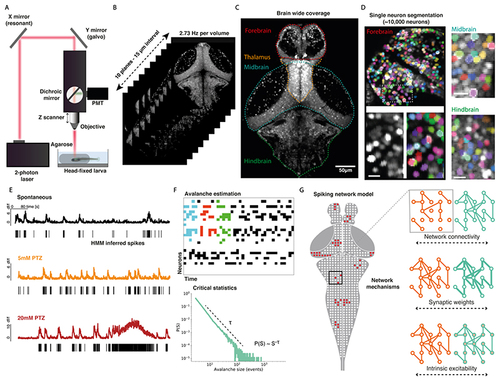
Study design.
(A) In vivo 2-photon imaging setup with head-fixed larval zebrafish. (B) Imaging was captured across 10 planes with 15 μm spacing at an imaging rate of 2.73 Hz per volume. (C) Max projection across 2 imaging planes of larval zebrafish volume taken with 2-photon microscope, demonstrating coverage of major brain regions. (D) Nuclear localised GCaMP fluorescence enables the segmentation of single neurons, as shown over exemplar forebrain (left), midbrain (top right) and hindbrain areas (bottom right) for a representative fish. The two images below the forebrain region show raw GCaMP signal (left) and segmented neurons (right) over a magnified area (scale bar is 10 μm). (E) Single cell traces shown from representative neurons for a single fish, showing normalised calcium fluorescence over time for spontaneous (black), 5mM PTZ (orange) and 20mM PTZ (red) conditions. A hidden Markov model (HMM) was used to infer spike times (black bars). (F) The spatio-temporal propagation of activity through the network was quantified as avalanches, as shown for 3 example avalanches (coloured by avalanche) for an example raster plot (top). Avalanche statistics were calculated to assess critical dynamics (bottom). (G) A network model of the larval zebrafish brain was constructed, which was used to test the role of specific network mechanisms in driving empirical avalanche dynamics. |

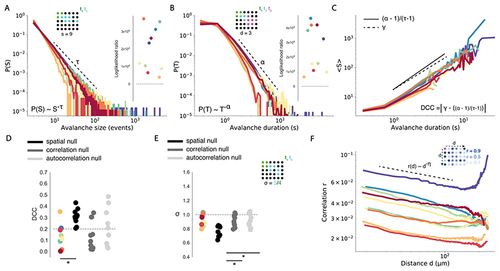
Avalanche estimation.
(A) Neurons exhibit on (red circles) and off (white circles) dynamics giving rise to ensembles that grow in space and time. (B) Hidden Markov model estimation of calcium transients showing normalised traces (blue), and estimated calcium transients (red). (C) Avalanche calculation legend. (D) For avalanches to begin, at least 3 nodes within the same neighbourhood must be active at t0. To propagate in time, any avalanche node active at t0 must also be active at t1. Once this step is satisfied, any nodes active at t1 that are connected via a neighbourhood to avalanche nodes at t1 become avalanche members. Avalanches terminate when no more nodes are active. Avalanche size (s) is the total number of activations and duration (d) is the number of time steps of the avalanche. |
Whole brain spontaneous neuronal activity exhibits critical statistics.
(A) Empirical distributions for avalanche size (S) with dotted line showing power law exponent T, and corresponding log likelihood ratio tests for power law versus lognormal distributions (right). Data points are coloured by fish. Avalanche schematic demonstrating the calculation of avalanche size s (top) for a single avalanche event, where coloured dots represent active neurons at tx. (B) Same as in (A), for avalanche duration (T) with exponent α. (C) The scaling relationship between S and T is shown by plotting mean S against T and fitting a linear regression line to estimate the exponent γ (dotted line). The exponent relation (α-1)/(τ-1) is calculated using avalanche exponents for S and T. DCC is calculated as the absolute difference between γ and (α-1)/(τ-1). (D) DCCs plotted for each fish against each null model (dotted line = critical threshold of DCC < 0.2). (E) Branching ratio σ plotted for each fish against each null model (dotted line = critical value of σ~1). Avalanche schematic demonstrating calculation of σ (right). (F) The quantity r(d), which estimates pairwise neuronal correlation as a function of distance, follows an approximate power-law with exponent η (dotted-line). Schematic demonstrating estimation of correlation (r) as a function of distance (d) (right). Magenta neuron is the neuron of interest. Other neurons are coloured by their correlation r to magenta neuron. * = p<0.01 |

Effect of avalanche parameters on critical statistics.
(A-D) Criticality statistics in spontaneous activity for increasing avalanche neighbourhood size k, over smaller (left, k = 0.04 – 0.23%; 10 – 19um) and larger ranges (right, k = 0.5 – 3.0%; 23 – 50um). (E-H) Criticality statistics in spontaneous activity for different minimum avalanche initiation sizes, from 2-4. |
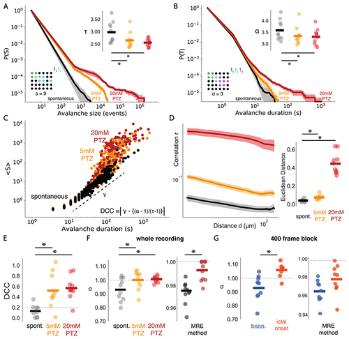
Seizures cause a loss of whole brain critical statistics.
(A) Complementary cumulative distributions for avalanche size (S), showing mean distributions across conditions (shaded regions represent the standard error), with power law exponents T compared (top right) across spontaneous (black), 5mM PTZ (orange) and 20mM PTZ (red) conditions. (B) Same as in (A), for avalanche duration (T) with exponent α. (C) The scaling relationship between S and T is shown by plotting mean S against T and fitting a linear regression line to estimate the exponent γ (dotted line), as shown for spontaneous (black), 5mM PTZ (orange) and 20mM PTZ (red) conditions. DCC is calculated as the absolute difference between γ and (α-1)/(τ-1). (D) The correlation function r(d) compared across conditions (left), with the Euclidean distance from fitted power laws plotted for each condition (right). (E) DCC compared across conditions. (F) The branching parameter σ plotted for each dataset across 30 minute recordings, using avalanche (left) and multiple-regression estimation approaches (right). (G) Same as in (F), for shorter 400 frame state transition periods, where baseline (base.) is before seizure transition and ictal onset is immediately following transition. * = p<0.01 |
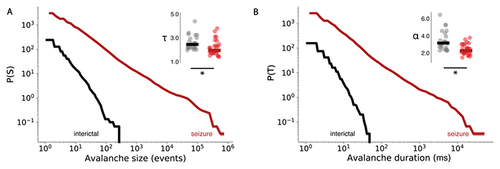
Human epileptic seizures at the macroscale alter avalanche dynamics.
Complementary cumulative distribution functions for avalanche size (A) and duration (B), comparing mean distributions across EEG datasets for inter-ictal (black) and seizure periods (red). Avalanche exponents are compared for avalanche size ( and duration (α) in interictal ( black bar = mean), and seizure (red bar = mean) conditions. |

Branching parameter assessed throughout seizure evolution.
The branching parameter σ was estimated using the avalanche approach across 1000 frames of generalised seizure periods in 10 frame bins. 2 datasets were excluded based on the absence of clear transitions from non-generalised to generalised activity, or insufficient frames following the transition initiation. σ remains close to 1 in the leadup to the generalised seizure and drastically increases as dynamics become highly synchronous, for most datasets (2, 3, 4, 5, 7, 8). Interestingly, following initial increases, σ quickly returns to ~ 1 while high synchrony is ongoing. Note that for some datasets (1, 6) σ remains close to 1 until after the onset of highly synchronous activity. Oscillatory dynamics following the peak of synchronous activity are characterised by moderate increases in σ above 1 (3, 7). |

Neuronal network mechanisms driving generalised seizure dynamics.
(A) Avalanche distributions from baseline, preictal and ictal-onset periods, alongside best model fits using all parameters. (B) Network connectivity schematic for sparse and dense networks (left). Best model fits using network connectivity parameter only, to pre-ictal (middle) and ictal-onset data (right). (C) Synaptic weights schematic for strong and weak synaptic weights (edge thickness = synaptic strength) (left). Best model fits using synaptic weights parameter only, to pre-ictal (middle) and ictal-onset data (right). (D) Intrinsic excitability schematic for high and low threshold to spike networks (red node = closer to spike) (left). Best model fits using intrinsic excitability parameter only to pre-ictal (middle) and ictal-onset data (right). (E) Model comparison for 3 parameter models (black), 2 parameter models (grey) and single parameter models (colours as above), for pre-ictal (middle) and ictal-onset data. The cost function used for model comparison was a regularised mean squared error term (left, See Methods). |

Increased connectivity drives the emergence of chaos in seizure networks.
(A) Using lagged coordinate embedding single variable (Y) can be used to reconstruct an attractor that is topologically equivalent to the full system, by using a series of delayed variables (Y, Yt-T, Yt-2T …, Yt-(m-1)T) of delay T and dimension m. Embedding each lagged variable into state space provides the reconstructed attractor, where tx is the position in state space at time x corresponding to the dotted red line (left). Isomap 3d embeddings of reconstructed attractors using lagged coordinate embedding for spontaneous (middle) and 20mM PTZ (right) data for a representative fish. (B) Schematic outlining the meaning of different λ values (top). Each colour represents the trajectory over time for a specific initial point along the attractor (high to low brightness represents movement in time). λ is the ratio of the difference between 2 points at the start (d0) and at t (dt). λ > 1: chaotic (red), λ < 1: stable (blue), λ = 1: neutral (green), where λ for each trajectory is calculated against the black trajectory. λ over time is compared for spontaneous and 20mM PTZ conditions (bottom), and mean λ is compared across spontaneous (black bar = mean) and 20mM PTZ conditions (red bar = mean) (top right). (C) λ over time compared for baseline and ictal-onset full parameter models (top), and λ over time is shown as a function of edge density m (bottom), ranging from pre-ictal values to ictal-onset values. Each line represents the mean λ over time for each model over 50 simulations. (D) Mean λ compared for baseline (base.) and ictal-onset full parameter models, and single parameter models (m = network connectivity, Vth = intrinsic excitability, r=synaptic strength) (top left). Correlation between m and mean λ is shown, ranging from pre-ictal values to ictal-onset values (bottom). Mean λ calculated using lagged coordinate embedding (LCE) on full parameter models across baseline (grey bar = mean) and ictal-onset models (crimson bar = mean) (top right). |
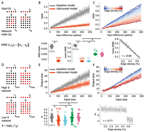
Increased connectivity disrupts the optimal network response properties of critical networks.
(A) For 2 similar inputs (i1 and i2) onto the network, the network mediated separation (NMS) is the Euclidean distance between the two corresponding network states (s1 and s2). (B) NMS is shown as a function of input difference compared for baseline and ictal-onset full parameter models (top). NMS slope and mean NMS is compared for baseline and ictal-onset full models and single parameter models (m = network connectivity, Vth = intrinsic excitability, r=synaptic strength) (bottom). (C) NMS as a function of input difference for increasing network connectivity m, ranging from pre-ictal to ictal-onset m values (top). Correlation between m and mean NMS (bottom). (D) For different inputs, the dynamic range δ is the log ratio of the input sizes (i1 and i2) that give rise to the largest and smallest network responses (Smax and Smin). (E) Output size as a function of input size compared for baseline and ictal-onset full parameter models (top). δ compared for baseline and ictal-onset full models and single parameter models (bottom). (F) Output size as a function of input size for increasing network connectivity m, ranging from pre-ictal to ictal-onset m values. Correlation between m and δ (bottom). * = p<0.01. |
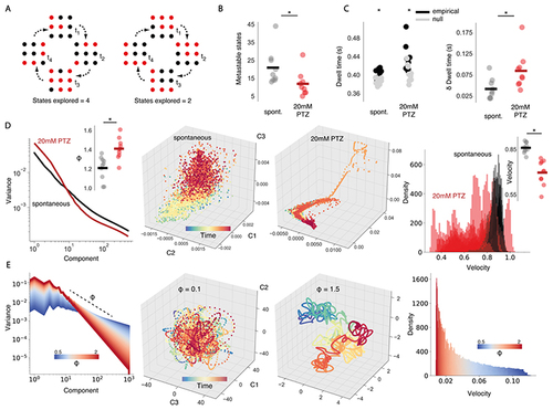
Generalised seizures cause sticky dynamics.
(A) A critical system can explore a greater subset of its possible brain states (left), while a non-critical system will explore a more limited subset (right). (B) The number of metastable states compared across spontaneous (black bar = mean) and 20mM PTZ conditions (red bar = mean). (C) Mean dwell time in each state compared across conditions, plotting both empirical and null model datapoints (left). Empirical dwell time minus null model dwell time (δ dwell time), as a measure of dwell time normalised to number of available states, compared across datasets (right). (D, left) Mean eigenspectrum function plotted across conditions, with Eigenspectrum slope ϕ plotted for each dataset (top right). (D, middle) 3d Isomap embedding of reconstructed attractor for an example fish. (D, right) State space velocity probability densities plotted for all fish, comparing spontaneous and 20mM PTZ conditions, with mean velocity compared across datasets (top right). (E, left) Simulated eigenspectrum function plotted for increasing ϕ. (E, middle) Random projection of eigenspectra into state space for different ϕ. (E, right) State space velocity probability densities plotted as a function of ϕ. * = p<0.01 |