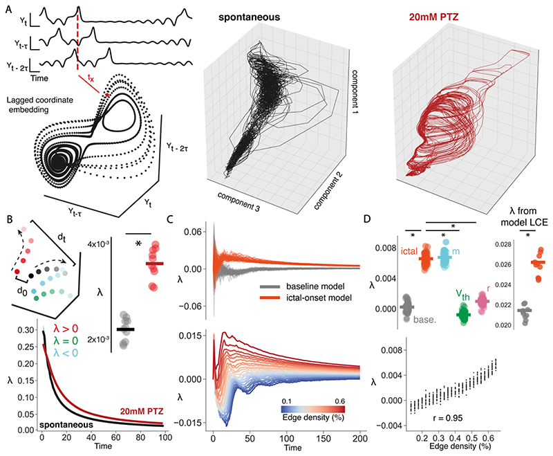
Figure 9

(A) Using lagged coordinate embedding single variable (Y) can be used to reconstruct an attractor that is topologically equivalent to the full system, by using a series of delayed variables (Y, Y_t-T, Y_t-2T …, Y_t-(m-1)T) of delay T and dimension m. Embedding each lagged variable into state space provides the reconstructed attractor, where t_x is the position in state space at time x corresponding to the dotted red line (left). Isomap 3d embeddings of reconstructed attractors using lagged coordinate embedding for spontaneous (middle) and 20mM PTZ (right) data for a representative fish. (B) Schematic outlining the meaning of different λ values (top). Each colour represents the trajectory over time for a specific initial point along the attractor (high to low brightness represents movement in time). λ is the ratio of the difference between 2 points at the start (d0) and at t (dt). λ > 1: chaotic (red), λ < 1: stable (blue), λ = 1: neutral (green), where λ for each trajectory is calculated against the black trajectory. λ over time is compared for spontaneous and 20mM PTZ conditions (bottom), and mean λ is compared across spontaneous (black bar = mean) and 20mM PTZ conditions (red bar = mean) (top right). (C) λ over time compared for baseline and ictal-onset full parameter models (top), and λ over time is shown as a function of edge density m (bottom), ranging from pre-ictal values to ictal-onset values. Each line represents the mean λ over time for each model over 50 simulations. (D) Mean λ compared for baseline (base.) and ictal-onset full parameter models, and single parameter models (m = network connectivity, Vth = intrinsic excitability, r=synaptic strength) (top left). Correlation between m and mean λ is shown, ranging from pre-ictal values to ictal-onset values (bottom). Mean λ calculated using lagged coordinate embedding (LCE) on full parameter models across baseline (grey bar = mean) and ictal-onset models (crimson bar = mean) (top right).