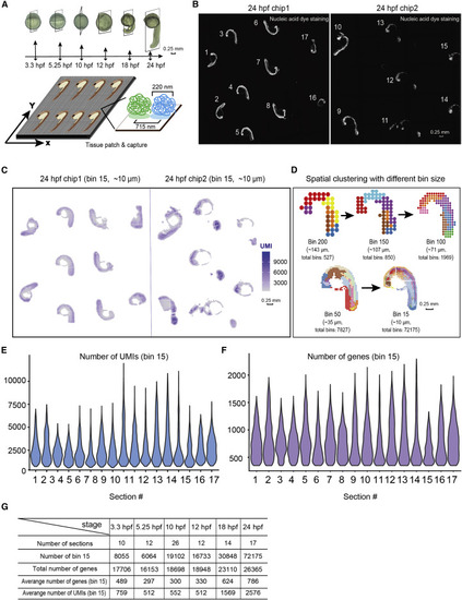
Figure 1. The Stereo-seq on multiple sections of the developing zebrafish embryos (A) Experimental outline (top): diagram of the zebrafish embryos and sagittal cryosections at different development stages which were subjected to Stereo-seq. Scale bars, 0.25 mm. Stereo-seq process diagram (bottom): the enlarged image shows the size of each spot and the distance between 2 adjacent spots. (B) Nucleic-acid dye staining of the 24-hpf zebrafish embryo sections attached on two 1-cm2 Stereo-seq chips. The number represents the serial number given to each section. Scale bars, 0.25 mm. (C) Spatial visualization of the distribution of captured transcripts (unique molecular identifiers [UMIs]) on all 24-hpf zebrafish embryo sections. Scale bars, 0.25 mm. (D) Unsupervised clustering of the 24-hpf zebrafish embryo section based on Stereo-seq data at different bin sizes. Scale bars, 0.25 mm. (E and F) Violin plot of the number of captured transcripts (E) and genes (F) of each 24-hpf zebrafish embryo section. (G) Table summarizing the numbers of sections used, total numbers of genes, total number of bins at bin-15 resolution, average captured number of UMIs, and genes at bin-15 resolution for each developmental stage in Stereo-seq.

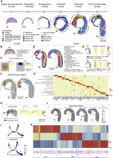
Figure 2. A spatial transcriptomic atlas of the developing zebrafish embryo (A) Unsupervised clustering of the zebrafish embryo section across sequential developmental stages analyzed by Stereo-seq at bin-15. Bins are colored by different regions. Scale bars, 0.25 mm. In this study, all sections from 10- to 24-hpf are displayed with head on the upper left and tail on the bottom right. The “#number” next to the sections represents the number given to each section, and all the sections in the following figures are marked with the “#number.” (B) Unsupervised clustering of the 3.3-hpf zebrafish embryo sections at bin-15. Bins are colored by spatial identities inferred from expressed marker genes. Scale bars, 0.25 mm. (C) The in situ hybridization images and the expression patterns of marker genes grhl3 and thy1 for superficial blastomere at 3.3-hpf. Scale bars, 0.25 mm. (D) Unsupervised clustering of the 24-hpf zebrafish embryo sections at bin-15. Bins are colored by spatial identities inferred from expressed marker genes. Scale bars, 0.25 mm. (E) Spatial visualization of indicated areas of the 24-hpf embryo on the left: detailed anatomical structures identified in the pronephros, and a combined structure including the spinal cord, the floor plate, and the notochord. The expression patterns of marker genes for each anatomical structure are shown on the right. Scale bars, 0.1 mm. (F) Unsupervised subclustering of the 24-hpf zebrafish nervous system. Bins are colored by spatial identities and cell types inferred from expressed marker genes. The subcluster colors are the same as the font colors of cluster names in (G). Scale bars, 0.25 mm. (G) Heatmap shows the mean expression level of marker genes between the indicated clusters of the zebrafish nervous system. (H) Spatial visualization of the hindbrain at 24-hpf, from left to right including indicated cell types and the expression of marker genes of different cell types. Scale bars, 0.25 mm. (I) Pseudotime analysis of hindbrain-related clusters as performed by Monocle 2. Bins are colored by cell types on the top (color legends of cell types are the same as those in Figure 2H) and colored by pseudotime stages on the bottom. (J) Spatial visualization of detailed structures of pseudotime states identified by Monocle 2 in the hindbrain on different sections at 24-hpf. Scale bars, 0.25 mm. (K) Heatmap shows the mean expression level of the top 30 DEGs different pseudotime states 1, 2, and 3. Representative genes related to each state are highlighted by red color.

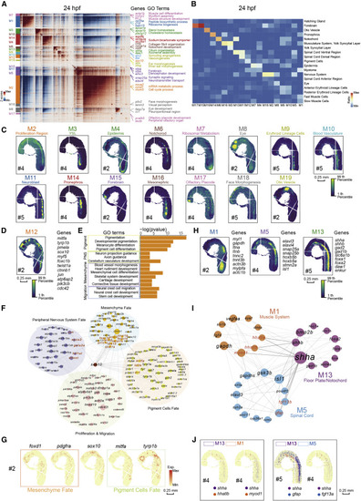
Figure 3. Spatial modules identified by hotspot uncover the interaction among spatial regions in 24-hpf zebrafish embryo (A) Heatmap shows the genes with significant spatial autocorrelation (12,675 genes, false discovery rate [FDR] < 0.05) grouped into 19 gene modules based on pairwise spatial correlations of gene expression in multiple sections of the 24-hpf zebrafish embryo. Selected genes and GO terms related to representative modules are highlighted on the right side. (B) Heatmap shows the ratio of the bins with high module scores (>3) in each module distributed in different spatial clusters, and the spatial clusters of the 24-hpf embryo are from Stereo-seq dataset in Figure 2D. (C) Spatial visualization of module scores for modules on 24-hpf embryo sections. Scale bars, 0.25 mm. (D) Spatial visualization of module 12 (M12). Scale bars, 0.25 mm. (E) Bar graph shows significantly enriched selected gene ontology terms in M12. (F) Protein-protein interaction (PPI) network of genes in M12. The network is visualized by Cytoscape. Node size represents the relative connectivity, and the TFs that interacted with sox10 are highlighted by red color. (G) Spatial expression pattern of genes in M12. These genes are related to the development of pigment cells fate (green), mesenchyme fate (orange), and sox10. Scale bars, 0.25 mm. (H) Spatial visualization of modules related to notochord/floor plate and neighboring tissues on 24-hpf embryo sections including M1, M5, and M13. Scale bars, 0.25 mm. (I) PPI network of interactive genes with shha/b in the three modules in Figure 3H. Representative genes are highlighted by red color. (J) Spatial expression patterns of shha and the interactive genes. Scale bars, 0.25 mm.

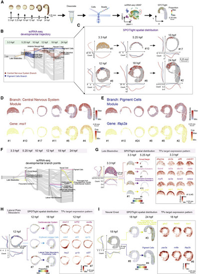
Figure 4. Construction of the spatially resolved developmental trajectories by integrated analysis of the scRNA-seq and Stereo-seq data (A) Schematic representation of the workflow for scRNA-seq of zebrafish embryos at different developmental stages using the C4 system and integrated analysis with a combination of the scRNA-seq and Stereo-seq data by applying SPOTlight. Scale bars, 0.25 mm. (B) Application of a Sankey diagram to visualize zebrafish embryo developing trajectory with scRNA-seq data. Two developmental branches which are developed from the presumptive ectoderm, namely, pigment cells, and central nervous system are simultaneously displayed on the Sankey diagram. (C) Application of SPOTlight to integrate Stereo-seq with scRNA-seq data to infer the spatially resolved developmental trajectories. Two developmental branches shown in (B) are simultaneously displayed on six sequential spatial sections to show the different spatial developmental trajectories. The graphs next to each section show bin counts distributions of corresponding cell types at two dimensions. The color legend is the same as that in Figure 4B. Scale bars, 0.25 mm. (D and E) Distribution of branch-specific gene module (top) and individual representative DEGs (bottom) of the central nervous system branch (D) and the pigment cells branch (E) on six sequential spatial sections. Scale bars, 0.25 mm. (F) Three selected developmental branch points at 3.3-, 12-, and 18-hpf. The late blastodisc (left), the lateral plate mesoderm (middle) and the neural crest (right), are shown in the Sankey diagram. (G–I) Cell-fate regulatory maps of different developmental destinations at 3.3-, 12-, and 18-hpf are related to Figure 4F. SPOTlight was applied to visualize the spatial distribution of cell subgroups with different differentiation together on one section (left) and separately on each section (middle); the graphs next to each section show bin counts distributions of corresponding cell types at both x and y axes (left). The spatial expression distributions of selected representative crucial TFs target genes are visualized on embryonic sections (right). Scale bars, 0.25 mm.

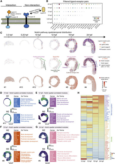
Figure 5. The relative spatial distance of different ligand-receptor pairs reveals the arrangement and interaction of signaling pathways (A) Model diagram of the analysis of ligand-receptor relative distance. (B) A dotted heatmap shows the expression scores and relative distance scores of ligand-receptor pairs that passed the filter (relative distance <5 bins in at least one time point, and correlation Pearson r > 0.5, p value < 0.05). (C) Spatial expression pattern of notch family genes (blue), deltal family genes (red), and jagged family genes (yellow) on embryo sections at the 6 time points (top). Spatial expression pattern of Notch receptors (red), ligands (blue) with a relative distances less than 2 bins, and the ligand-receptor pairs expressed in the same bin (purple) (middle). Spatial expression pattern of Notch target genes (red) on the embryonic sections at different time points (bottom). Scale bars, 0.25 mm. (D–G) Gene modules identified using hotspot show spatial correlation with Notch pathway in 10- (D), 12- (E), 18- (F), and 24-hpf (G) embryos. Module scores are plotted on the left, and selected genes and GO terms related to spatially correlated modules are highlighted on the right. Scale bars, 0.25 mm. (H) A heatmap shows the temporal expression changes of genes selected from modules in Figures 5D–5G.