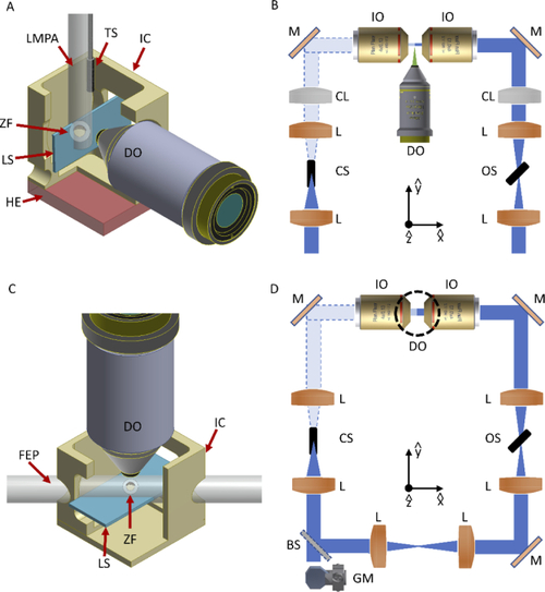
Schematic of the LSFM mounting and scanning methods used. (A) The zebrafish embryo (ZF), within its chorion, is embedded inside a lmpa cylinder hanging from the top of the imaging chamber (IC) and connected to a translation-rotational stage, to enable the scan through the vertical light-sheet (LS). The emitted photons are collected by the detection objective (DO). A heating element (HE) is integrated below the chamber, while a temperature sensor (TS) is immersed in the imaging medium to monitor the temperature for the whole experiment. (B) Schematic of the illumination optical path for the first LSFM setup. Each of the two illumination arms contains two lenses (L) and a cylindrical lens (CL) for the LS formation. After reflection on a mirror (M), the illumination objective (IO) generates the vertical LS in the sample plane. The illumination paths also contain two shutters (CS = closed shutter, OS = open shutter), that are employed to block the light from one of the two arms, generating the alternate illumination scheme. (C) A FEP tube crosses at 45° the imaging chamber, creating a fluidic circuit through which the embryo is loaded and then positioned in the FoV of the detection objective. Once here, the entire chamber (and the attached FEP tube) is displaced vertically to scan the sample across the horizontal LS. The imaging chamber models are here sectioned to ease visualization of the interior part. (D) Schematic of the illumination optical path for the second LSFM setup. A galvanometric mirror (GM) generates the LS that through a beam-splitter (BS) is sent to each illumination objective, to create the horizontal LS at the sample plane. The dotted circumference denotes the position of the vertical detection objective. Shutters are again used to implement the double alternate excitation scheme. x? and ? denote the horizontal plane, while z? denotes the vertical axis.

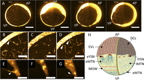
LSFM permits to see the microtubule re-arrangement in the whole embryo. (A) dclk2-GFP embryo during synchronous mitosis events of the blastomeres. Lateral view, AP = animal pole, VP = vegetal pole, scale bar 200 µm. (B) Normalized mean intensity profile over time of the blastoderm region as highlighted in (A). The overlaid bars indicate the subsequent developmental stages of the embryo, from 256-cell to sphere stage. (C) The obtained graph for the normalized mean intensity over time on the yolk surface (circular ROI in (A)). Overlaid bars highlight drops of intensity corresponding to MOW passages. (D-F) Three frames (maximum intensity projection) from time-lapse LSFM imaging of the same embryo. The white circumferences indicate the wavefront of the same MOW that is advancing over the eMTN of a dclk2-GFP embryo at cleavage stage, vegetal view. During time, the wavefront travels toward the vegetal pole of the embryo (the travelling is indicated by the reducing size of the overlapped circumference). See also Visualization 1. MC = marginal cell, scale bar 200 µm. Central black region is due to the LS bending caused by the curvature of the sample. (G-I) Zoom in at the square region highlighted in (D), visualizing the eMTN (G) before (diffuse network), (H) during (sparser MTs), and (I) shortly after (re-diffused network) the MOW passage. Scalebars 50 µm.

Temporal concurrence of mitosis and MOWs. (A-C) Visualization of blastomere/eYSN cycle phases (relative ROI indicated in panel (G)) through microtubules? labelling: (A) metaphase, (B) interphase, (C) metaphase (at minutes 9, 24, 102). Scale bars 25 µm. (D-F) Visualization of MOWs passages in the subsequent yolk region (relative ROI indicated in panel (G)). The MT network is (D) highly oriented and sparse, then (E) re-diffuses, and again (F) sparse (at minutes 15, 27, 108). Scale bars 25 µm. (G-H) The same dclk2-GFP embryo from a lateral view at three different timepoints (at minutes 9, 24, 102), scale bars 200 µm. Animal pole at top left, vegetal pole at bottom right. Arrows indicate expansion (pointing outward in A and C) and contraction (pointing inward in B) of the blastoderm margin. (J) Normalized mean intensity graph visualizing blastomeres/YSNs cycles (metaphases are peaks, interphases are valleys, graph obtained from the local analysis). (K) Normalized mean intensity graph visualizing the periodic MOWs passage (arrows) over the yolk region (graph obtained from the local analysis). (L) The periodic blastoderm contractions (valleys) and expansions (peaks). Blastoderm margin expansion and nuclei metaphase appear to be synchronized, MOW passage follows after few minutes. See Supplement 1 for details on how the graphs were retrieved. See also Visualization 2.

MOWs depend on the cell/eYSN divisions. (A-B) Internal slices from the 3D stack showing the YSN (white arrow) before (A) and during (B) a mitotic event. (C-D) Maximum intensity projection for the same area in (A-B), showing the MT network emerging from the YSN, before (denser network, C) and after (sparser network, D) the YSN mitotic event. Scale bars 50 µm. (E) Normalized mean intensity profiles of three YSN tracked through the 3D stack over time, recording their last two divisions (overlaid bars). For better visualization, an incremental offset is applied to avoid graphs? overlapping. (F) Normalized mean intensity profile from a 19 µm ROI (white circumference in (C)) over the MT branch from the maximum intensity projection over time. The retrieved graph records the last two MOWs? initiations (overlaid bars), corresponding to the YSN divisions in (E). (G) Time points at which mitosis (squares) and MOWs? initiations (circles) happens, for embryos at different temperatures. Each letter identifies one embryo. (H) Violin plots resuming the effect of experimental temperature on periodicities of mitosis (left part) and MOWs? initiations (right part). p-values: ns = p>0.05, *= p<0.05, **= p<0.01, ***= p<0.001, ****= p<0.0001. (I) Overview on the 63 analysed [mitosis/MOW initiation] coupled events and their outcome to the hypothesis ?MOW initiation coupled with mitosis?. (J) Correlation graph between the number of detected MOW initiation and of detected cell/YSN divisions from each embryo (letters). Dotted line represents identity line. See also Supplement 1 Fig. S2.

MOWs? global visualization and analysis. (A) Left panel: representation of the coordinates system and spherical coordinate convention of the double-hemisphere 3D model for the zebrafish embryo. Pv is a general point over the spherical yolk surface, and P?v its projection on the xy plane. Right panel: exemplification of meridians (black) and parallels (blue) on the blastoderm (mb, pb) and yolk sphere (my, py). In both panels, the red circumference represents the blastoderm margin. AP = animal pole, VP = vegetal pole, BM = blastoderm margin. (B) Maximum intensity projection of LSFM imaging of a dclk2-GFP embryo, lateral view, and some of the paths followed to adapt the analysis to the spherical yolk shape. Scale bar 200 µm. (C) Normalized mean intensity kymograph relative to a single meridian of the yolk sphere, over time. Intensity drops (red arrows) reveal MOWs? passage from BM to VP. Speed calculation is performed through slope measurement (elevation angle/time). (D) Some of the paths followed to perform the analysis over the blastoderm hemisphere. Scale bar 200 µm. (E) Normalized mean intensity kymograph relative to a single meridian of the blastoderm hemisphere, over time. Intensity peaks (arrows) reveal the mitotic wave passage from AP to BM. From comparison of (C) and (E) is shown how MOWs follow in time the mitosis but also, in this particular embryo, the presence of an outlier as one mitosis (black arrow in E) is not followed by any MOW. (F) Over the maximum intensity projection of the same embryo (scale bar 200 µm), the analysis along parallels is performed. This produces the normalized mean intensity kymographs relative to blastoderm (G) and yolk (H), showing the wavefronts (dotted lines) of the mitotic waves (G, black dotted line indicates the outlier) and MOWs (H).

Internal MT network morphology. (A) Depth-coded projection of a z-stack in which the information relative to the outer YCL was digitally removed. The internal microtubule network and its extension within the yolk is visible. Visualized depths range between 0 µm (white) and 350 µm (blue). Vegetal view, left and right images of the embryo are stitched together, scale bar 200 µm. (B) Maximum intensity projection over a 40 µm range of a yolk section. The internal MTs forms circular patterns (white arrows) and also are connected to the external yolk MTs (eMTN) network. Vegetal view, left and right images of the embryo are stitched together, scale bar 200 µm. (C) Zoom (single slices) on the yolk surface, showing clear connections between the internal and external MT networks (white arrows, upper and lower panel), and interconnections between internal MTs (white arrow, lower panel). Scale bars 50 µm. (D) Embryo at sphere stage, lateral view. AP = animal pole, VP = vegetal pole, scale bar 200 µm. (E) zoom into the ROI indicated by * in (D), single slice, showing connection of internal MTs to an eYSN (white arrows). eMTN = external MT network, scale bar 50 µm. (F) Maximum intensity projection over a 20 µm range of the same ROI showing also the extension toward the internal portion of the yolk of the MT connected to an eYSN. Scale bar 50 µm. See also Visualization 5. (G) zoom into the ROI indicated by ** in (D), single slice, showing an internal MT bundle (white arrow) extending perpendicular to the image plane. (H) Maximum intensity projection showing the end point of that internal MT bundle, coinciding with a centriole (white arrow) associated to an eYSN. (I) An XZ re-slice view of the same ROI showing the connection of the same MT bundle and its extension toward the interior of the yolk. Scale bars 50 µm. See also Visualization 4. All figures relative to dclk2-GFP embryos, and Orange HOT lookup table was used to ease iMTN visualization.

Internal MT network dynamics. (A) Time series visualizing a maximum intensity projection over a 30 µm of a developing embryo from (left to right) blastula, 50%, 70%, and 90% epiboly. The iMTN is visible in all these stages. AP = animal pole, VP = vegetal pole. Left and right images of the embryo are stitched together, scale bars 200 µm. See also Visualization 6. (B-D) Time series visualizing through maximum intensity projection over 26 µm the dynamics of iMTN-eMTN connections upon MOW passage. Before MOW passage the connection is clearly visible (white arrow, B), during MOW passage the connection is lost (C), and is re-established after MOW passage (white arrows, D). Scale bars 50 µm. See also Visualization 7. Single slice images relative to the same frame of (B) and (D) are visible in Supplementary Fig. S4. (E-G) Time series visualizing the XZ re-slice dynamics of iMTN-eYSN connection upon eYSN mitosis. Before the eYSN division the connection is present (E), during the division the connection is lost (F), and re-established after the division is completed (G). Scale bars 50 µm. All figures relative to dclk2-GFP embryos, and Orange HOT lookup table was used to ease iMTN visualization. (H) Updated model for the MT networks populating the zebrafish yolk between 512-cell and sphere stages. On the left side, the eMTN associated to the eYSN is subject to the MOW travelling toward the VP, exemplified as a belt of low-density MT. On the right side, the section view of the embryo is illustrated. The iMTN is present within the whole yolk cell. EVL = enveloping layer, DCs = deep cells. Representation not in scale.