ZFIN All Figures, Dokmegang <i>et al.</i>, 2021

Dokmegang et al., 2021

ZDB-PUB-210325-11
PMID:33760050
Fig. 1.
Fig. 2.
Fig. 3.
Fig. 4.
Fig. 5.

FIGURE SUMMARY

Title: Quantification of cell behaviors and computational modelling show that cell directional behaviors drive zebrafish pectoral fin morphogenesis
Authors: Dokmegang, J., Nguyen, H., Kardash, E., Savy, T., Cavaliere, M., Peyriéras, N., Doursat, R.
Source: Full text @ Bioinformatics

Fig. 1.

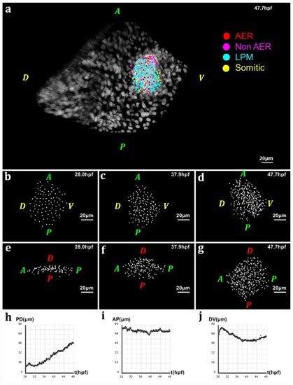
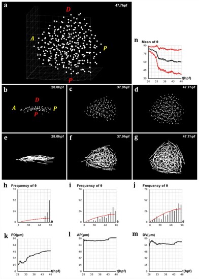
Geometry of the pectoral fin based on live imaging and image processing data. (a) 3D rendering of raw data nuclear staining at 𝑡=47.7 $t = 47.7$ hpf: dorsal view of the zebrafish body with detection of approximate nuclear centers of the pectoral fin cells highlighted by colored dots, where the color code depends on the cell type; scale bar: 20 μm. (b–d) After applying cell detection methods: 3D rendering of the approximate nucleus centers of LPM cells in the pectoral fin at different stages of development, respectively 𝑡=28 $t = 28$ hpf, 𝑡=37.9 $t = 37.9$ hpf and 𝑡=47.7 $t = 47.7$ hpf (AP: anteroposterior axis; DV: dorsoventral axis). (e–g) 3D rendering of the pectoral fin at the same times along the AP axis and PD axis. (h–j) Evolution over time of the fin size in μm along the PD, AP and DV axes respectively. Fin expansion occurs mainly along PD. It undergoes a slight compaction along the other two axes, more pronounced along the DV axis

Fig. 2.

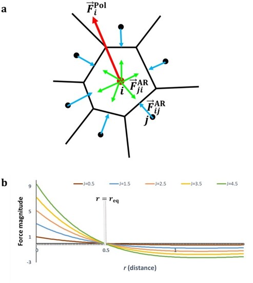
Center-based computational model of multicellular dynamics. (a) Schema of a local cell neighborhood and the abstract forces on cell centers. 𝐹→AR𝑗𝑖 ${\vec{F}}_{j i}^{AR}$ is the passive AR force exerted on a cell i by a cell j. 𝐹→Pol𝑖 ${\vec{F}}_{i}^{Pol}$ is the active migration force driven by the cell’s polarity (specified in Section 3.4). (b) Plot of the Morse force profile (derivative of the Morse potential) defining 𝐹→AR ${\vec{F}}^{AR}$ , for different parameter values. This curve presents two regimes: a positive regime (attraction) below an equilibrium distance 𝑟eq $r_{eq}$ and a negative regime (repulsion) above

Fig. 3.

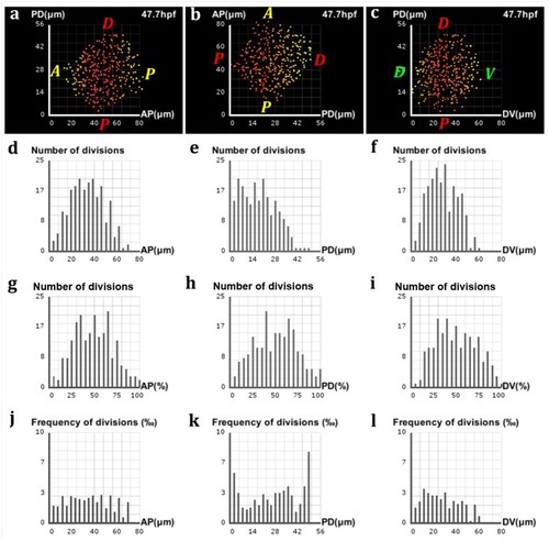
Analysis of proliferation in the zebrafish pectoral fin. (a–c) Frequencies of divisions along the AP, PD and DV axes respectively, highlighted by a yellow-red color gradient coding for differences in proliferation rates across the fin. (a, c) The preponderance of red at the center of the fin shows where the bulk of cell divisions takes place, with only a few of them occurring near the lateral surfaces (yellow). (b) A decreasing gradient of proliferation rates from the proximal pole to the distal tip characterizes the PD axis. (d–f) Marginal distributions of proliferation along the AP, PD and DV axes respectively, expressed in numbers of cells with respect to the absolute distance in μm along the axis. (g–i) Same distributions with respect to the relative distance on the axis. (j–l) Same distributions expressed in proportions of cells with respect to the absolute distance

Fig. 4.

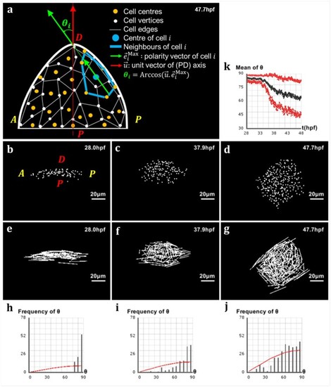
Analysis of directional cell behaviors in the zebrafish pectoral fin. (a) Schematics in 2D of the method used to analyze directional cell behaviors: for each cell i, θ_i denotes the polarity angle that this cell forms between its elongation axis 𝑒→Max𝑖 ${\vec{e}}_{i}^{Max}$ (extracted from the maximum eigenvalue of the covariance matrix of its neighborhood 𝒩𝑖 $N_{i}$ ) and the PD axis 𝑢→ $\vec{u}$ . (b–d) Lateral view of the pectoral fin at different stages of development, respectively 𝑡=28.0 $t = 28.0$ hpf, 𝑡=37.9 $t = 37.9$ hpf and 𝑡=47.7 $t = 47.7$ hpf. (e–g) Vector field of the cells’ elongation axes 𝑒→Max𝑖 ${\vec{e}}_{i}^{Max}$ in the pectoral fin at the same stages. (h–j) Distribution of the polarity angles θ_i of the cells in the pectoral fin at the same stages, compared with the standard distribution of random angles formed by two arbitrary vectors in 3D (red curve). (k) Evolution over time of the average polarity angle 𝜃⎯⎯ $\bar{θ}$ of the fin cells ± its standard deviation Δθ $Δ θ$ shown in red

Fig. 5.

Simulation of pectoral fin morphogenesis based on directional cell behaviors. Values of the equation parameters: λ=0.2,ν=1.6,𝐽=0.001 $λ = 0.2, ν = 1.6, J = 0.001$ . (a) 3D view of the simulated fin at the final stage 𝑡=47.8 $t = 47.8$ hpf. (b–d) Lateral view of the simulated fin at different stages of development, respectively 𝑡=28.0 $t = 28.0$ hpf, 𝑡=37.9 $t = 37.9$ hpf and 𝑡=47.7 $t = 47.7$ hpf. (e–g) Vector field of the cells’ elongation axes 𝑒→Max𝑖 ${\vec{e}}_{i}^{Max}$ in the simulated fin at the same stages. (h–j) Distribution of the polarity angles θ_i of the cells in the simulated fin at the same stages, compared with the standard distribution of random angles formed by two arbitrary vectors in 3D (red curve). (k–m) Evolution over time of the simulated fin size in μm along the PD, AP and DV axes respectively. We observe roughly the same behavior as the real fin in Figure. 1h–j. (n) Evolution over time of the average polarity angle 𝜃⎯⎯ $\bar{θ}$ of the simulated fin cells ± its standard deviation Δθ $Δ θ$ shown in red. This curve is more scattered than Figure 4k

Acknowledgments

This image is the copyrighted work of the attributed author or publisher, and ZFIN has permission only to display this image to its users. Additional permissions should be obtained from the applicable author or publisher of the image. Full text @ Bioinformatics

Dokmegang et al., 2021 ZDB-PUB-210325-11 PMID:33760050

Quantification of cell behaviors and computational modelling show that cell directional behaviors drive zebrafish pectoral fin morphogenesis

Dokmegang et al., 2021

ZDB-PUB-210325-11
PMID:33760050