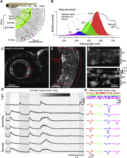
Recording from RGC Dendrites and Somata In Vivo

(A) Schematic of Islet2b:mGCaMP6f expression in RGCs (green) across a section of the larval zebrafish eye, with somata in the ganglion cell layer (GCL) and dendrites in the inner plexiform layer (IPL); see also Figures S1A–S1C. INL, inner nuclear layer.

(B) Average spectrum of natural daylight measured in the zebrafish natural habitat from the fish’s point of view along the underwater horizon (solid line). Convolution of the zebrafish’s four cone action spectra with this average spectrum (shadings) was used to estimate the relative power each cone surveys in nature, normalized to red cones (100%). Stimulation LED powers were relatively adjusted accordingly (“natural white”).

(C and D) GCaMP6f expression under two-photon surveyed across the entire eye’s sagittal plane (C) and zoom-in to the strike zone as indicated (D). Within the zoomed field of view, a curved scan path was defined (“banana scan”) to follow the curved GCL and IPL for activity recordings (E), which effectively “straightened” the natural curvature of the eye.

(E and F) Example activity scan with RGC dendrites occupying the top part of the scan in the IPL and somata occupying the bottom part in the GCL as indicated (E) and correlation projection [41] of activity following white noise stimulation highlighting responding regions in the scan alongside example regions of interest (ROIs) (F; see also Video S1).

(G) Mean (black) and individual repeats (gray) example responses of ROIs from (E) to full-field stimulation as indicated.

(H) As (G), now showing linear kernels to red, green, blue, and UV components recovered from natural white noise stimulation (STAR Methods).

Note that several ROIs display a robust UV component despite the ~20-fold attenuated stimulation power in this band relative to red (B). See also Figures S1D–S1G.

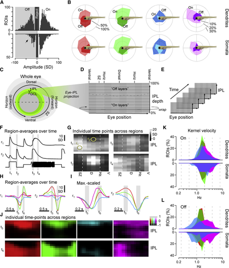
Major Functional Response Trends across the Eye

(A) Kernel amplitudes of all dendritic (top) and somatic (bottom; y-flipped) ROIs, shown for the maximal amplitude kernel of each ROI irrespective of color. For a breakdown by color, see Figures S2G and S2H. The arrowhead emphasizes a relative reduction in OFF responses at the level of somata. Chi-square with Yates correction for On:Off distributions dendrites versus somata: p < 0.00001.

(B) Prominence of different color and polarity responses among dendrites (top row) and somata (bottom row), plotted across visual space. In each case, all kernels that exceeded a minimum amplitude of 10 SDs were included. Scale bars in percent of dendritic/somatic ROIs that were recorded in a given section of the eye such that the percentages of On, Off, and non-responding (<10 SD) add to 100% are shown.

(C–E) Schematic illustrating how dendritic ROIs from different parts of the eye and IPL depth (C) were mapped into a 2D “Eye-IPL” map (D), which can then also be analyzed over time (E). Note that this involved “cutting” the circular range of eye positions such that the ventral retina is represented at either edge along the 2-projections’ x axis.

(F and G) Example snapshots of mean responses to chirp stimulation (cf. Figure 1G) mapped into an eye-IPL map as schematized above (C–E). Data can be plotted as time traces for a given region of the eye and IPL (F; r_1,2 as indicated in G) or alternatively as a time-frozen snapshot of activity across the eye and IPL at different points in time (G; t_1–4 as indicated in F). See also Videos S2 and S3.

(H–J) As (F) and (G) but instead showing mean kernels across the four spectral wavebands, where (H) and (I) are mean and max-scaled mean kernels for Eye-IPL regions r_1,2 (as in F), respectively. (J) shows each kernel’s full Eye-IPL map at two time points t_5,6 as indicated in (H) and (I) (see also Figure S2I). In the color scale bar, 0 equates to the baseline of each bin’s kernel and 1/−1 to their respective maximum or minimum (cf. I). See also Video S4.

(K and L) Distribution of central frequencies (STAR Methods) of dendritic (top) and somatic (bottom; inverted y axis) kernels in the four wavebands, separated into On (K) and Off (L) kernels. Wilcoxon rank-sum test, 1 tailed with correction for multiple comparisons for all pairwise comparisons between same polarity distributions of spectral centroids, is shown. Dendrites: all p < 0.001 except R_Off versus G_Off (p = 0.0011) and G_On versus B_On (p = 0.69). Somata: all p < 0.001 except R_On versus U_On (p = 0.00101), R_Off versus G_Off (p = 0.033), G_On versus B_On (p = 0.045), B_On versus U_On (p = 0.064), R_On versus B_On (p = 0.25), and R_On versus G_On (p = 0.57).

Diverse Color Opponencies in RGCs

(A) Each dendritic (top) and somatic (bottom; inverted y axis) ROI that passed a minimum response criterion (STAR Methods) was allocated to a single bin in a ternary classification scheme according to the relative polarities of their four spectral kernels (3 response states On, Off, and no response) raised to the power of 4 spectral channels (red, green, blue, and UV): 3⁴ = 81 possible combinations. The central row between the bar graphs indicates each bin’s spectral profile: “On” (red, green, blue, and UV); “Off” (black in the respective row); and no response (white in the respective row). For example, the leftmost group, which comprised the highest number of dendritic ROIs, corresponds to ROIs displaying Off kernels in red, green, and blue, with UV showing no response. The bar graphs are color coded as follows: dark gray (non-opponent Off); light gray: (non-opponent On); and orange/brown (opponent). Brown bins indicate opponent bins that are only classified as opponent because they comprise a Blue-Off component (see main text). The horizontal insets summarize all ternary response groups that exceeded a minimum size (indicated by the dashed line) across the following categories: Off; On; and Opponents, here divided into types of spectral computations as indicated by the color circles; two-color symbols denote “simple” opponencies (single spectral zero crossing, e.g., red versus green) between the indicated wavebands (red, green, blue, and UV), although the “flower” symbol denotes complex opponencies (>1 spectral zero crossing, e.g., red and blue versus green).

(B) Maximum-amplitude scaled average kernels of the ten most abundant spectral classes among dendrites in (A).

(C and D) Dendritic groups from (A) summarized according to their position in an Eye-IPL map (cf. Figure 2). (C) summarizes major groups: Off (left, top) and On non-opponent (left, bottom); opponent (right, top); and On+Off non-opponent (right, bottom). (D) As (C), with opponent groups divided into their specific spectral computations as indicated. Note that most specific functions in (C) and (D) are restricted to specific regions of the eye and IPL. For example, green versus blue simple opponent computations occur mostly in the ON layers of the ventral retina that survey the world above the fish (D, bottom left).

Functional Clustering of Dendritic ROIs

(A–F) Dendritic ROIs from across the entire eye were clustered based on their four spectral kernels (STAR Methods) to yield a total of n = 15 functional clusters that comprised a minimum of 10 ROIs. Shown are heatmaps of red, green, blue, and UV kernels (A, from left to right, respectively) and associated mean chirp response (B), with each entry showing a single ROI, followed by each cluster’s Eye-IPL projection (C), each mean kernel (D), max-scaled kernels superimposed (E), and the mean chirp response (F). Error shadings in SD are shown. For clarity, low-amplitude mean kernels were omitted from column (E). Note that C₁₁^∗ comprised a mixture of responses and may comprise a variety of low-n functional RGC types. Grayscale color maps (A–C) were linearly equalized by hand to maximize subjective discriminability of the full response range across the population of all recordings in a dataset. Lighter grays indicate higher activity/kernel amplitudes. For corresponding data on somata, see Figure S3.

(G) Summary of cluster distributions across the eye, irrespective of IPL depths, for dendritic (top) and somatic (bottom) clusters, scaled by their relative abundance (in %; see scale bars). Eye-distribution profiles were manually allocated to one of the following groups based on which part of visual space is mainly surveyed: SZ (dendritic C₁; somatic C₂); forward (dendritic C₅; somatic C₃); outward (dendritic C_3,9; somatic C_9,11); horizon (dendritic C_2,11; somatic C₁,₄,₁₀); up (dendritic C_4–8; somatic C₇); and down (dendritic C_10,12–15; somatic C₁₂,₁₃). Two large clusters (somatic C_5,8) did not obviously fit to any of these categories and were instead grouped separately as “mixed.” It is possible that these clusters comprise several smaller groups of functional RGCs with distinct eye-wide distributions.

(H) As (E) for both dendritic (top) and somatic (bottom) data, but with all spectral kernels in each waveband superimposed. Note kinetic similarities across most red and green kernels and near complete absence of positive deflections in blue kernels.

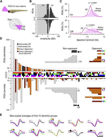
RGC Circuits in the Strike Zone

(A) A second series of RGC imaging experiments as shown in Figures 1, 2, 3, and 4 was performed, this time exclusively recording from the strike zone (SZ), which surveys visual space above the frontal horizon.

(B) Overview of dominant On and Off responses among dendrites (top) and somata (bottom) for the SZ. Dendrites n = 2,370 On, n = 624 Off; somata n = 1,312 On, n = 379 Off. Chi-square with Yates correction for On:Off distributions dendrites versus somata: p < 0.22. For details, cf. Figure 2A; for a breakdown by color, see Figures S4A and S4B.

(C) Relatively slowed central frequency tuning of SZ-UV kernels (lines) compared to the retina average of UV kernels (filled) among both On (top) and Off (bottom) kernels (cf. Figures 2K and 2L). Both p < 0.0001, Wilcoxon rank sum test, 1 tailed.

(D) Ternary spectral classification of SZ dataset (for details, cf. Figure 3). Overall, note the striking On dominance and increased presence of UV responses in this dataset.

(E) Maximum amplitude scaled average kernels of the ten most abundant spectral classes among dendrites in (D).

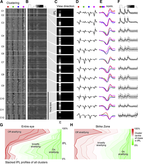
The SZ Is Dominated by Broadly Stratifying UV-Sensitive On Clusters

(A–F) Clustering of dendritic ROIs from SZ dataset (for details, cf. Figures 4A–4F). Note that all clusters except for C₁₂ are dominated by On kernels, with C_1–3 showing pronounced UV responses despite the relatively low UV-signal power in the stimulation light (cf. Figure 1B). For corresponding clustering of SZ somata, see Figure S5.

(G and H) Side-to-side comparison of functional stratification profiles of clusters from data across the eye (G; cf. Figure 4C) and from SZ only (H; cf. C). In each case, all cluster stratification profiles of a dataset were sorted by their center of mass in the IPL (from 100%: Off to 0%: On), stacked on top of each other, and normalized to the number of ROIs per IPL depth. In addition, profiles were color coded by their center of mass in the IPL as indicated. Note that most SZ clusters (H) tended to broadly cover much of the IPL with a center of mass near the middle of the IPL (white), although eye-wide stratification profiles (G) instead showed a greater tendency to stratify in either Off (red) or On (green) layers.

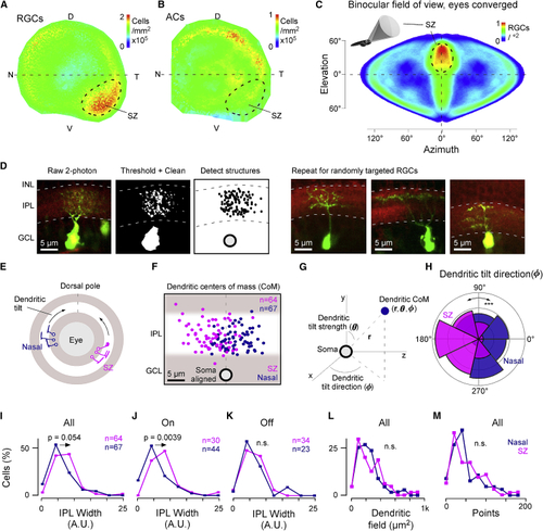
Elevated RGC Density and Relative Overrepresentation of Diffuse ON-RGCs in the SZ

(A and B) Density maps of all RGCs (A) and ACs (B) computed from cell counts in Figures S6A–S6C, from n = 1 retina. D, dorsal; N, nasal; SZ, strike zone; T, temporal; V, ventral.

(C) Projections of RGC densities from (A) into binocular visual space during hunting (eyes converged), as illustrated in the inset. Note that the two SZs neatly superimpose (see also [27]).

(D) Illustration of photoconversion and pre-processing pipeline for digitizing single RGC morphologies. Left: following photoconversion, cells were imaged as stacks under two-photon (green) in the background of BODIPY staining to demarcate the IPL borders (red). Cells were then thresholded and manually “cleaned” where required prior to automatic detection of image structures and alignment relative to the IPL borders. The resultant “point clouds” were used to determine summary statistics of each cell (e.g., E–M) and were also projected into density maps for visualization (Figure S6G). Right: three further examples of photoconverted RGCs are shown.

(E–M) A total of n = 64 and n = 67 randomly targeted RGCs from the SZ and nasal retina, respectively, were processed for further analysis, which included computation of their dendritic tilt (E–H), stratification widths within the IPL (I–K), en face dendritic field area (L), and total number of detected dendritic structures (“points”; M; STAR Methods). The dendrites of nasal (purple) and SZ (pink) RGCs both tended to tilt toward the eye’s dorsal pole (E: schematic; F: soma-aligned data of all dendrites’ center of mass). Dendritic tilt was quantified in soma-centered polar coordinates based on the Cartesian x,y,z coordinates that emerge from the original image stacks (G), such that r: distance in microns between soma and dendritic center of mass (Figure S6D), θ (0°:90°): strength of the dendritic tilt (0° and 90° denoting no tilt and maximal positive tilt, respectively; Figure S6E), and ϕ (0°:360°): direction of the dendritic tilt in approximately retinotopic space (approximate as the eye is curved). ϕ significantly differed between nasal and SZ RGCs (H). For summarizing widths, RGCs were considered as a single group (I) or split into On and Off RGCs (J and K, respectively), based on the IPL depths of their dendritic center of mass (here, the upper third of the IPL was considered “Off” and the bottom two-thirds were considered “On”). Kolmogorov-Smirnov test for circular statistics (H) and Wilcoxon rank sum test, 1 tailed (I–M), is shown.