
- Title
-
Motor context dominates output from Purkinje cell functional regions during reflexive visuomotor behaviours
- Authors
- Knogler, L.D., Kist, A.M., Portugues, R.
- Source
- Full text @ Elife
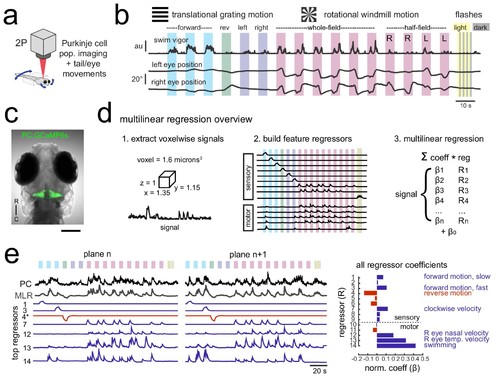
Using population imaging and multilinear regression to describe feature responses across the Purkinje population during visuomotor behaviors. (a) Cartoon of the embedded zebrafish preparation under the two-photon microscope with freely-moving eyes and tail. (b) Overview of the visual stimuli presented to the awake, behaving zebrafish during volumetric two-photon calcium imaging. See Materials and methods for further details. The mean swimming activity and eye position for a representative fish across an entire experiment is shown (N = 100 trials). (c) Composite bright field image of a seven dpf zebrafish larva from a dorsal view showing Purkinje cells expressing GCaMP6s driven by a ca8 enhancer element. Scale bar = 100 microns. (d) Overview of the multilinear regression analysis. See Materials and methods for additional details and see Figure 1—figure supplement 1 for full list of regressors. (e) Left panels, example calcium signal from a Purkinje cell across two planes (black trace) can be well recapitulated through multilinear regression (MLR, grey trace; R2 = 0.77). The regressors with the seven largest coefficients (β) are shown below scaled in height and colored by their β value (blue = positive, red = negative). The asterisk for regressor four refers to a negative value of β which results in an inverted regressor. Right, a bar graph quantifying the normalized β values for all regressors for this cell with the regressors shown at left labelled. See also Figure 1—figure supplements 1 and 2. |

Functional imaging anatomy and full regressor list.(a) Single imaging planes showing PC:GCaMP6s fluorescence as obtained from confocal imaging (upper panel) and during two-photon experiments (middle panel). Lower panel, a single confocal imaging plane from a PC:NLS-GCaMP6s fish where GCaMP is restricted to the nucleus. Red arrowheads indicate example Purkinje cell somata. Scale car = 25 microns. (b) Quantification of Purkinje cells in the entire cerebellum at seven dpf as counted in the PC:NLS-GCaMP6s line. N = 3 fish. (c) The complete set of regressors used in analysis of calcium imaging data. Individual regressors fall into one of five categories (three sensory and two motor), as indicated by the categories at right. Tail and eye motor regressors are calculated for each imaging plane based on the motor activity during that trial, therefore a representative example from one trial in the dataset is shown here. See also Videos 1 and 2 for example imaging trials with the sequence of visual stimuli displayed. (d) Projections of the first ten principal components of Purkinje cell activity in response to experimental stimuli across all fish (N = 6; see Materials and methods), ordered in increasing variance explained. Components that show a high degree of anatomical clustering are colored. Colors are arbitrarily chosen. |

Calcium signals report complex spikes reliably but can also report simple spike bursts.(a) Example cell-attached electrophysiological recording (ephys, black trace) and simultaneously recorded fluorescence trace (green) from a Purkinje cell expressing GCaMP6s under the Purkinje cell-specific ca8 enhancer. All complex spikes (orange dots) are accompanied by an increase in fluorescence as shown as a deflection in the fluorescence trace that accounts for every peak in the complex spike regressor (orange trace, spike rate convolved with GCaMP kernel). In contrast, only high frequency bursts of simple spikes (blue dots) influence the fluorescence signal (indicated by blue arrowheads). (b) The mean spike-triggered fluorescence signal and standard deviation is plotted for the example cell from a) for complex and simple spike bursts (N = 25 each). (c) A composite epifluorescent image showing a bright field dorsal view of the cerebellum together with single-cell GCaMP expression in the Purkinje cell from the previous panels and the rhodamine-filled electrode contacting this cell. The outline and midline of the cerebellum is indicated by the dashed white line. Scale bar = 50 microns. (d) The mean spike-triggered fluorescence signal and standard error is plotted for eight cells (N = 6 fish) for complex and simple spike bursts. (e) The relative contribution of the complex spike (CS) and simple spike (SS) regressors (spike rates convolved with the GCaMP kernel) to the fluorescence signal in each cell as determined by least squares regression (see Materials and methods) across the eight cells. The example cell from a) is indicated. (f) The location of all example cells, color-coded by relative SS regressor contribution. (g) Overview of i) the morphology of a singly-labelled Purkinje cell and the subcellular regions of interest (ROIs) with ii) corresponding calcium signals obtained from high resolution two-photon imaging (see Materials and methods). Scale bars = 20 microns. (h) Quantification of the correlation coefficient between the calcium signal from the most distal dendritic segment and the soma. N = 5 cells from three fish. |
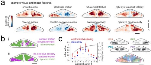
Purkinje cell activity is functionally clustered across the cerebellum.(a) Heatmaps of the z-projected mean voxelwise correlation coefficients from multilinear regression (MLR) with example sensory and motor regressors for a representative fish (see Materials and methods). Scale bar = 50 microns. (b) Voxels from the example fish in a) are colored according to whether the best regressor for correlated sensory stimuli and motor events (including i) swimming and ii) eye movement) are sensory (magenta), motor (green), or equal/uncorrelated (white). (c) Left, quantification of principal component analysis, clustering, and stereotypy of Purkinje cell responses. Left axis, index values across the first ten principal components with respect to the anatomical clustering of principal components within a fish (red line) and the stereotypy of these clusters across fish (blue line). Dotted black line shows an index value of 1 (equivalent to chance). Right axis, total variance explained across principal components. Right panel, mean spatial mapping of the four principal components with the highest index values for anatomical clustering and stereotypy as individual maps (above) and composite (below). Colors are arbitrarily chosen. |
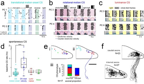
Purkinje cells in different regions show complex spike responses that encode different visual features and one group sends outputs to a different downstream region.(a) Raster plot (upper left panels) and histogram (lower left panels, 500 ms bins) of complex spikes occurring across trials during translational whole-field motion of black and white bars in all four cardinal directions for two example Purkinje cells (PC). Numbers assigned to PCs for this and panels b-c are arbitrary. (b) Raster plot (upper left panels) and histogram (lower left panels, 100 ms bins) of complex spikes occurring across trials during whole- and half-field bidirectional rotational motion of a black and white windmill for an example cell. The dashed lines over the histogram show the velocity of the stimulus in each direction across the trial. (c) Raster plot (upper left panels) and histogram (lower left panels, 100 ms bins) of complex spikes occurring across trials during whole-field light/dark flashes for two example cells, (i) and ii). (d) A box plot of complex spike firing rates during blank trials (no visual stimuli) for cells grouped by their sensory or motor complex spike category (see Figure 2). N = 31, 14, 5, 8. Asterisks indicate significance (one-way ANOVA with Bonferroni post hoc correction, p<0.001). j (i) The location of cells colored by complex spike phenotype are plotted onto a flattened dorsal view of the cerebellum with all coordinates flipped to the right half of the cerebellum. e (ii) Three example maximum projection images of traced axonal morphology from stochastically-labelled, Fyn-mClover3-expressing Purkinje cells for which electrophysiological recordings were also obtained. Labels for each cell refer to the electrophysiological traces in panels a-c. The asterisk for cell a) indicates that these coordinates were flipped to the right half of the cerebellum. Scale bar = 50 microns. e (iii) Categorical grouping of complex spike phenotypes for internal versus caudal axonal projections. N = 17 cells from 17 fish. (f) Morphed Purkinje cell axonal morphologies from single-cell labelling across fish (N = 50 cells) can be grouped into two populations based on axonal projection (as for e iii). N = 27 cells with internal axons, N = 23 cells with caudal axons. |

Purkinje cell dendrites show a mostly planar morphology.(a) Four example Purkinje cell morphologies obtained by single-cell labeling (see Materials and methods) are shown with their soma and axon in black and dendrites in orange. Asterisks indicate a truncated axon. (b) Quantification of dendritic morphology as measured by determining the principal axes (see Materials and methods) shows that dendrites are significantly more planar than chance (p<0.01, Wilcoxon signed rank test). |
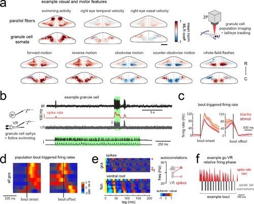
Granule cells across the cerebellum code for motor activity with high fidelity.(a) Heatmaps of the z-projected mean voxelwise correlation coefficients of two-photon granule cell GCaMP6s signals from multilinear regression with example sensory and motor regressors averaged across seven fish (see Materials and methods). Scale bar = 50 microns. Upper right, cartoon of experimental set-up. (b) Left, cartoon of experimental set-up. Right, upper panel, example cell-attached recording from a granule cell (gc, upper trace, black) from a blank trial with simultaneous ventral root recording (VR, lower trace, gray). The granule cell firing rate is also shown (spike rate, middle trace, orange). The bout highlighted in green (i) is shown below on an expanded timescale. (c) The bout on- (left) and off- (right) triggered mean firing rates for this granule cell during blank recordings (orange) and stimulus trials (red). (d) Z-scored heatmaps of bout on- (left) and off- (right) triggered mean firing rates in all granule cells sorted by mean firing rate in the 300 ms following bout onset (N = 8 cells from eight fish). (e) Mean autocorrelation heatmap for spikes (upper panel) and ventral root recordings (VR, lower panel) for all granule cells from d), sorted by time to first peak in the VR autocorrelation. The red arrowheads signify granule cells with significant spike autocorrelations during fictive swim bouts (N = 3; p<0.001, Ljung-Box Q-test; see Materials and methods). Right, the first significant peak in the VR autocorrelation for each recording is plotted to give the mean fictive swim frequency for each fish. The red circles are the mean spike autocorrelation frequency obtained from the three significantly autocorrelated granule cells. (f) An example bout from the cell indicated in e), which was located ipsilateral to the ventral root recording. The smoothed spike rate (red) is in antiphase with the ipsilateral fictive tail contractions (grey). |