Measuring high-spectral resolution tuning curves in zebrafish bipolar cells

(A) Schematic of the larval zebrafish retina, with cone terminals in the outer retina and bipolar cell (BC) terminals in the inner retina highlighted.

(B) Mean calcium responses of red-, green-, blue-, and UV-cone terminals to a series of 13 spectrally distinct widefield flashes of light as indicated (data from Yoshimatsu et al.²⁷). Note that, for clarity, the response to a 14^th “low-power-control” UV LED was graphically removed compared to the original publication.

(C–F) Illustration of recording strategy for BC terminals in the inner plexiform layer (IPL) and exemplary results. An optical triplane approach (C, top) was used to simultaneously record from three planes of larval zebrafish BC terminals expressing SyjGCaMP7b by way of two-photon imaging coupled with remote focusing (STAR Methods). From here, we automatically placed regions of interest (ROIs) and detected the boundaries of the IPL (D; STAR Methods). Time traces from all ROIs in a recording plane were Z scored and averaged across 3–5 response repeats of the full stimulus sequence (E). Example traces from individuals ROIs (F) are shown as individual repeats (gray) and averages across repeats (black).

Zebrafish larva schematic (A) by Lizzy Griffith. See also Figure S1.

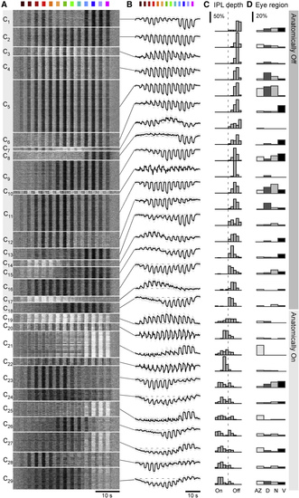
Clustering into 29 functional BC types

Overview of the result from unsupervised clustering of all BC data recorded as shown in Figure 1 that passed a minimum quality index (QI) (QI > 0.4; STAR Methods). For each cluster, shown are the individual BC mean responses as heatmaps (A); the corresponding cluster means and SD shadings, with approximate baseline indicated in dashed (B); distribution of ROI positions in the IPL (C); and each cluster’s distribution across the four recording regions within the eye (D, from left: acute zone; dorsal; nasal; and ventral). Histograms in (C) are area normalized by cluster and in (D) by recording region. Clusters are ordered by their average anatomical position in the IPL, starting from the border with the inner nuclear layer (cf. C). The colored symbols indicate the overall spectral group as assigned later (cf. Figures 5F–5K).

Reconstructing bipolar cell responses from cones

(A–E) Summary of the reconstruction strategy for example cluster C₂₂ (for details, see STAR Methods). Each BC-cluster reconstruction is based on the linear combination of the spectral tuning functions of the four cone types (A; from Yoshimatsu et al.²⁷) with four stereotyped temporal components associated with individual light flashes (B), yielding 4 × 4 = 16 weights (C). Weights are shown in blocks of temporal component weights (from left: light transient; light sustained; dark transient; and dark sustained) associated with each cone (indicated by the corresponding colors). Bars above zero indicate sign-inverted (“On”) weights, while bars below zero indicate sign-conserved (“Off”) weights. The corresponding full expansion of this reconstruction is shown in (D). Individual combination of each cone’s tuning function (A) with each temporal component (B), scaled by their corresponding weight (C), yields sixteen “sub-traces” (D; upper four traces in each of the four panels, labeled L_tr, L_sus, D_tr, and D_sus). Summation of each cone’s four sub-traces yields that cone’s total contribution to the cluster (D, bottom traces, labeled “sum”). Finally, summation of the four cone totals yields the full reconstruction (E, black trace), shown superimposed on the target cluster mean (gray).

(F) As (A)–(E) but showing only the weights (top), cone totals (middle), and full reconstructions (bottom) for another four example clusters (from left: C₁; C₁₅; C₁₄; and C₂₅).

Further detail on reconstructions is shown in Figure S2, and all clusters’ individual results are detailed in Data S1.

A functional overview of cone bipolar cell mappings

Overview of all BC-cluster means (A, gray traces; cf. Figure 2B) and their full reconstructions based on the strategy detailed in Figure 3 (black traces). Associated weights are shown in (B). For clarity, “near-zero” weights (abs(w) < 0.5) are omitted. Full weights are shown in Data S1. Note that, based on outer retinal inputs only, weights are generally expected to be sign conserving for clusters in the traditional Off layer (C₁–C₁₈) and sign inverting in the anatomical On layer (C₁₉–C₂₉), as indicated on the right. The round symbols plotted next to each cluster (A) denote their allocated spectral group, as detailed in Figures 5F–5K and associated text.

Major trends in cone weights and spectral tunings

(A and B) Histograms of all weights associated with inputs to each of the four cones across all clusters, independent of temporal-component types (A) and, correspondingly, histograms of all weights associated with temporal components, independent of cone type (B). Near-zero weights (abs(w) < 0.5) are graphically de-emphasized for clarity. All weights contributed equally to these histograms, independent of the size of their corresponding cluster.

(C–E) Scatterplots of all clusters’ weights associated with each cone plotted against each other as indicated. Large symbols denote the mean weight associated with each cone and cluster across all four temporal components (i.e., one symbol per cluster), while small symbols denote each weight individually (i.e., four symbols per cluster, corresponding to L_tr, L_sus, D_tr, and D_sus). The remaining three possible cone correspondences (G:B, G:U, and B:U) are shown in Figures S3A–S3C.

(F–K) Peak-normalized “bulk” spectral tuning functions of all 29 clusters, grouped into six categories as indicated. The strength of each line indicates the numerical abundance of ROIs belonging to each cluster (darker shading = larger number of ROIs; exact number of ROIs contributing to each cluster are listed in Data S1). As appropriate, spectral tuning functions of cones (cf. L) are shaded into the background, as appropriate (G and H, thick colored traces) to illustrate the close spectral correspondences of associated cones and BCs. Similarly, for three spectrally opponent groups (I and K), the approximate positions of the corresponding cone’s zero crossings are indicated with a vertical shaded line (cf. L).

(L) Cones’ spectral tuning functions, with approximate zero crossings (blue and green cones) and zero positions (red and UV cones) graphically indicated.

(M and N) Histograms of zero crossings across all BC clusters, incorporating the abundance of ROIs belonging to each cluster. Shown are crossings of bulk spectral tunings functions (M; cf. F–H) and of spectral tuning functions that were computed for each temporal component individually, as indicated (see also Figures S3F–S3I and Data S1). Note the three prominent peaks of zero-crossing positions, approximately aligned with the zero positions and crossings of the cones. These peaks largely disappeared when time components were fully randomized (Figure S3D) or randomly permuted across cones (Figure S3E).

Cone-weight distribution across the inner plexiform layer

Two-dimensional histograms of weights (x axes) associated with each cone resolved by IPL position (y axes). Brighter colors denote increased abundance. For simplicity, the weights associated with the light (L_tr and L_sus) and dark components (D_tr and D_sus), are combined in (A) and (B), respectively. Moreover, near-zero weights are not shown (central white bar in all panels). The thick white dotted lines indicate approximate expected distribution of weights based on traditional “On-Off” lamination of the inner retina. By each panel’s side, instances where this expectation is violated are highlighted as “polarity violation.”

Possible links across vertebrate retinal color circuits

Conceptual summary schematics of retinal circuits for color vision in zebrafish (A); dichromatic mammals, such as many rodents (B); and some trichromatic old-world monkeys, such as humans (C). The colored “graphs” indicate approximate spectral tuning functions of retinal neurons in a given layer, as indicated.