
- Title
-
A parameter-free statistical test for neuronal responsiveness
- Authors
- Montijn, J.S., Seignette, K., Howlett, M.H., Cazemier, J.L., Kamermans, M., Levelt, C.N., Heimel, J.A.
- Source
- Full text @ Elife
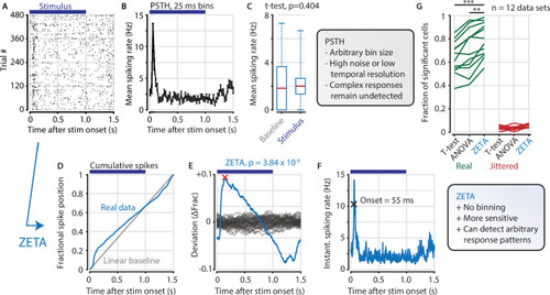
(A,B) Raster plot (A) and PSTH (B) for a neuron that shows an onset peak and a reduced sustained spiking in response to a visual stimulus (purple bars). (C) A common approach for computing a neuron’s responsiveness is to perform a t-test on the average activity per trial during stimulus presence (0–1 s) and absence (1.0–1.5 s), which fails to detect this neuron’s response (paired t-test, p = 0.404, n = 480 trials). (D) ZETA avoids binning, by using the spike times to construct a fractional position for each spike (blue) and compares this with a null-distribution of a stationary rate (grey). (E) The difference between the real and null curves gives a deviation from expectation (blue), where the most extreme value is defined as the Zenith of Event-based Time-locked Anomalies (ZETA, red cross). To compute its statistical significance (here, p = 3.84 × 10⁻⁹), we compare ZETA to the variability over repeats of the procedure with jittered onsets (grey curves). (F) A ZETA-derived instantaneous spiking rate allows a reliable estimation of response onset. (G) At a significance threshold of α = 0.05, ZETA detects more stimulus-responsive cells than both a mean-rate t-test (***: paired t-test, p = 2.8 x 10⁻⁷, n = 12 data sets) and an ANOVA over bins using an optimal bin width (**: p = 0.0014).
|

(A) Spikes were recorded with neuropixels in mouse V1 and aligned with the onset of square-wave drifting gratings. (B) Applying the ZETA-test, we found that 93.3 % of all V1 neurons showed significant firing rate modulations that were time-locked to stimulus onset. Using a rate-based t-test between stimulation (0–1 s) and no stimulation (1–1.5 s) epochs across trials registered 77.3 % of neurons to be visually responsive. Neurons detected by only ZETA are green, by both methods are blue, by only a mean-rate t-test are red, and by neither are grey. Arrows indicate the neurons shown in C. (C) Two example neurons that are (1) detected by a rate-based t-test as well as ZETA (top) and (2) not detected by a rate-based t-test, but only by ZETA (bottom). (D) We investigated the false-positive rate of both approaches by jittering the onsets of visual stimuli; this preserved the temporal structure of the spiking response, but destroys the time-locked modulations in activity. (E–F) same cells and analyses as in B-C but for jittered onsets. Red indicates neurons included by ZETA, but not a t-test; green indicates neurons included by a t-test, but not ZETA. As expected, the percentage of false positives (i.e., neurons with ζc/z-statistic > 2.0) was around 5 % (α = 0.05) for both approaches. Note the change in axis magnitude from B to E.
|
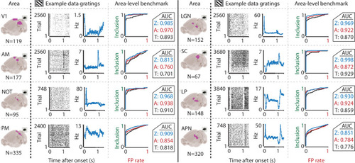
We recorded neuronal responses to drifting gratings (1 s with 500 ms blank ITIs) from various visual brain areas: V1, SC, AM, LP, NOT, APN, PM, and LGN. For each area, we show an example neuron’s raster plot (left) and binned responses (right). All cells depicted here were significant using ZETA. Area-level benchmark summaries show ROC analyses of the inclusion rate (y-axis) and false-positive (FP) rate (x-axis) for ZETA (Z, blue), bin-wise ANOVA (A, red), and rate-based t-tests (T, black). In all cases, the AUC of the ZETA-test exceeded both the ANOVA’s AUC and t-test’s AUC.
|
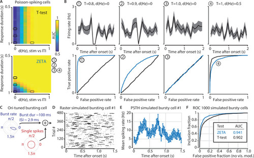
(A) Top: the ability of the t-test to differentiate simulated stimulus (non)modulated cells depends only the total spike count during stimulus (0–1 s) and inter-trial interval (ITI, 1–2 s) periods (x axis; firing rate difference d(Hz)), but not on the duration of the cell’s response when keeping the spike count constant (y axis; response duration T). Bottom: in contrast, the ZETA-test can differentiate stimulus modulation using either variable. (B) Top: example PSTHs of single cells corresponding to the markers 1–4 in (A). Bottom: ROC curves for the combination of variables marked as 1–4 in (A). The ZETA-test always exceeds the t-test’s performance, except for a limited range where the response duration is 1 s. (C) A more biologically plausible test case is bursting neurons that have an elevated probability of bursting during stimuli. (D–E) This simulation produces no ‘onset’ peaks of activity that the ZETA-test can exploit. (F) However, despite the lack of clear peaks of activity, the ZETA-test exceeds the t-test’s ability to detect stimulus-modulated bursting cells (ZETA AUC = 0.941, t-test AUC = 0.902).
|
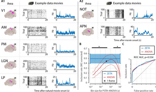
(A) We recorded neuronal responses to natural movies (four scenes that repeated every 20 s) from various visual brain areas: V1, AM, PM, LGN, LP, NOT, and APN. For each area, we show an example neuron’s raster plot (left) and binned responses (right). All cells depicted here were significant using ZETA. (B) We determined a neuron’s responsiveness using a 1-way ANOVA over all binned responses (i.e. PSTH-level ANOVA) for various bin sizes and MC-corrected (black) and using the ZETA-test (blue). Note that the ZETA-test is timescale-free and plotted at all x-values only for easy comparison with the ANOVAs. Curves show mean ± SEM over brain regions (n = 7). ZETA shows an inclusion rate similar to the most optimal bin sizes (0.0333s – 0.2667s), and significantly higher than bin sizes of 0.0167 s or shorter, as well as 0.533 s or longer (*, FDR-corrected paired t-tests, p < 0.05). (C) An ROC analysis on all n = 977 cells showed that the ZETA-test and a combined set of ANOVAs were similarly sensitive (ZETA-test AUC: 0.792 ± 0.011; ANOVAs AUC: 0.798 ± 0.010; z-test, p = 0.554).
|
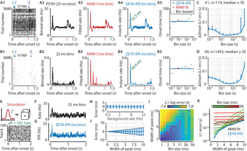
(A,B) Responses of two example V1 cells to drifting gratings. From left to right: (1) Raster plots showing the estimated onset latency (‘L’, green), and times of ZETA (blue) and –ZETA (purple). (2) Spiking rates using 25 ms bins. (3) Spiking rates using multiplicative inhomogeneous Markov interval (MIMI) model-based fits. (4) Binning-free instantaneous spiking rates provide a much higher temporal resolution. Using the first crossing of half-peak firing rates, we determined the onset latencies of these cells to be 52.5 and 59.4 ms. (5) Estimated onset times using our method for instantaneous firing rates (blue), MIMI model-based fits (red), or PSTHs with bin widths from 0.1 to 100 ms (black). Onset latency estimates depend on the chosen bin size, and the optimal size varies across cells. (C–D) The median (± SE) difference in onsets estimated by our instantaneous firing rates compared to that of various sized bins for V1 cells (C, n = 119) and for cells from all brain regions (D, n = 1403). Both C and D show the onsets estimated by the two methods were most similar for bin sizes between 1–10 ms. (E–K) Benchmarking of peak detection using artificial Poisson neurons that show a transient peak. (E) Example Poisson cell for a background rate of 10 Hz and a peak-width of 10 ms. With the true peak at 100 ms, the estimation error here was 1.1 ms. (F) Binning the cell’s spiking response in 25 ms bins reduces the peak height and temporal precision. (G) Our instantaneous spiking rate preserves a sharper peak response and allows for a temporally accurate latency estimation. (H) The detection of peak latencies is insensitive to realistic levels of a stationary Poisson background firing rate (13 base rates, 0.5–32 Hz). (I) The mean error is unbiased, and the standard deviation in the onset peak latency estimate scales linearly with the width of the peak. Dotted lines show the real peak width. Graphs in H-I show mean ± sd. (J) The error in peak latency estimation depends on both the bin width and the width of the neuron’s peak response. Red crosses indicate the bin size with the lowest error for a given peak width. (K) Plotting the latency estimation error shows that different bin sizes (red-green) are optimal for different peak-widths. The accuracy of the latency obtained from MIMI-based fits (black) is less sensitive to the peak width, but never performs as well as well as the most optimal bin size. The error based on our binning-less IFR (blue) is as at least as low as the most optimal bin size, for any peak width.
|
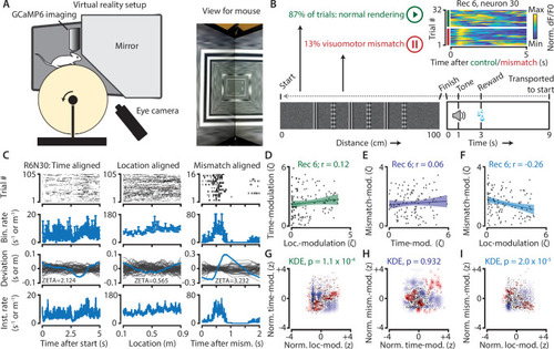
(A) Schematic of setup showing mouse on running wheel (lhs) viewing a virtual tunnel (rhs). (B) Trials consist of a 100 cm linear track. One second after the mice ran to the end of the tunnel, an auditory stimulus signaled that a water reward would be delivered two seconds later. 6 s after reward delivery, mice were transported to the start of the virtual tunnel. In a subset of trials, the rendering of the tunnel was paused at a random location, eliciting a visuomotor mismatch signal. Top right shows calcium imaging data for an example ‘mismatch neuron’ during 16 control and 16 mismatch trials. (C) Spiking data for example neuron obtained from exponential fits of the dF/F0 signals. Putative spikes were aligned to start (left), location of the animal on the track (middle), or mismatch onset (right). From top to bottom: raster plot of putative spike times; mean ± SEM of firing rates over trials (n = 105 trials, of which n = 16 mismatch trials); spiking deviation underlying ZETA; instantaneous firing rate. (D–I) Relationship between time-, location-, and mismatch-modulation. One point is one neuron. (D–F) ZETA-scores for example recording 6 (N = 120 neurons). (G–I) Analysis using a kernel-density estimate (KDE) to test whether joint-encoding of two features is more common than expected by chance (see Figure 1). (G) More neurons showed joint-encoding of both spatial and temporal location than expected by chance (p = 1.1 × 10⁻⁴). (H) Joint-encoding of temporal location and mismatch was not significantly different from chance (p = 0.932). (I) Location on the virtual track and visuomotor mismatch are less likely to be encoded by the same neuron than expected from chance (p = 2.0 × 10⁻⁵). See Figure 7—figure supplement 1 for more details on the KDE procedure.
|
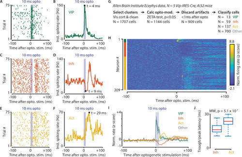
(A–F) Response of example cells classified as VIP (A,B), Inhibited (C,D) and Activated (E,F). (G) Data were recorded in visual cortex from 5 Vip-Cre mice at the Allen Brain Institute. Cells were only included if the clustering quality was sufficient (1707 cells total). A ZETA-test included cells that were modulated within (–0.5, + 0.5 s) after optogenetic stimulation (N = 1144 cells). IFR peak- and trough-latency was computed and cells were discarded if their peak was earlier than 1 ms after optogenetic stimulation onset. Remaining cells were classified as VIP (N = 13), Inhibited (N = 59), Activated (N = 137), or Other (N = 700). (H) Heat map showing normalized firing rate of VIP (top), Inhibited (middle), and Activated (bottom) cells. (I) Mean ± SEM of PSTH (2.5 ms bin size) over all VIP (green), Inhibited (orange), Activated (yellow), and Other (gray) cells. (J) Inhibited cells showed significantly lower mean IFR-peak latencies after optogenetic stimulation than Activated cells (Inh: 17.4 ms; Act: 23.0 ms; Mann-Whitney U-test, p = 5.1 × 10⁻⁷).
|