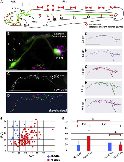
The lateral line in larval zebrafish (A) Schematic representation of a larval zebrafish showing neuromasts (red circles) of the anterior (ALL) and posterior (PLL) lateral line. Posterior neuromasts are named (L for troncal and Ter for terminal), and the planar polarization of their constituent hair cells (horizontal or vertical) is indicated (red arrowheads). Lateralis afferent neurons (LANs) and the lateralis central lintel (LCL) are shown in green. (B) Confocal image of a HGn39D transgenic larva (green) injected with Sill:mCherry (red), showing the neuronal soma of a posterior LAN (pLAN) within the posterior ganglion (PLLG) and its position within the LCL. The anterior ganglion (ALLG) is also shown. (C) Structure of the central projection of an individually marked LAN. (D) Skeletonization of the same projection shown in (C) with terminal varicosities marked with colored dots. (E–I) Skeletonized central arbors of the same neuron over consecutive days from 2.5 to 6.5 days-post fertilization (dpf). In all panels, anterior is left and dorsal is up. (J) aLANs and pLANs (respectively, blue diamonds and red squares) constitute distinguishable morphological classes according to the number of anterior and posterior varicosities (respectively AVs and PVs). (K) Bar chart showing significant differences between aLANs (blue) and pLANs (red) for AVs and PVs. aLANs have similar number of AVs and PVs along the length of the central projection. Scale bars are 50 μm. See also Figure S1.

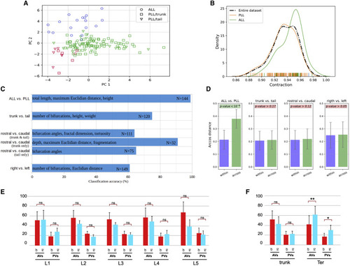
Morphometric analysis and classification of LANs (A) Distribution of original neuron type labels projected onto the first two principal components (PC) according to unsupervised Gaussian Mixture Models clustering based on morphometrics. The only clear alignment is with a 2-class separation, which matches ALL (aLANs) and PLL (pLANs). (B) Probability distribution functions of Contraction values (which measure neuronal branch tortuosity or meandering) for the whole cell population and for ALL and PLL neurons separately. The ALL and PLL distributions correspond to the peak of the bimodal Contraction distribution, confirming discrete rather than continuum classes. (C) Classification accuracy (expressed as percent correct on the horizontal scale) for distinguishing between various subsets of axonal projections based on their morphometric parameters. The most discriminant features are reported in each case along with the sample size corresponding to each grouping. (D) Persistence diagram vector analysis demonstrates that only aLANs/pLANs arcosine distances were statistically smaller within classes than across classes. (E) Comparison of the number of AVs and PVs between caudorostral pLANs (crpLANs, red) and rostrocaudal LANs (rcpLANs, blue). (F) Comparison of AVs and PVs between crpLANs (red) and rcpLANs (blue) in LANs from L1 to L5 analyzed as a whole (L1-L5_pLANs) and terminal LANs (Ter-LANs). See also Figure S2 and Video S1.

Lateral-line topographic map and rheotaxis (A and B) Volume-filled skeletons of 6 pLANs morphed onto a reference brain. Each pLAN innervates a different neuromast: L1 (red), L2 (green), L3 (blue), L4 (cyan), L5 (magenta) and Ter (yellow). (A) Side view and (B) top view. The central projections crossed one another along the length of the hindbrain. (C) Scheme of a double injection of a larval zebrafish with magenta and red dextrans, in HGn39D (green). Magenta dextran is injected into the L2 neuromast to label only L2_pLANs. The red dextran is injected into the terminal neuromasts to label only Ter_pLANs. (D) Maximal projection of the central projections of pLANs labeled with magenta and red dextrans, showing with corresponding-color arrowheads the central projections of L2_pLANs and Ter_pLANs relative to one another. The somata of the labeled neurons are indicated with color-coded arrowheads. Note that somatotopy is not precise along the LCL. (E) Scheme of the projections shown and color-coded in (D). (F and G) Central projections of a red- and a magenta-labeled axon within the background of the HGn39D transgenic line that labels the LCL with EGFP (green) (F). Color-coded arrowheads indicate the relative position of each axonal projection along the LCL (G). (H and I) Same specimen after the severing and regeneration of the peripheral axons, revealing that central axons do not change relative position along the somatotopic axis despite peripheral rewiring (I). (J) Orientation of intact and manipulated specimens at 6dpf under no flow (left hand-side, or under laminar water flow at 6mm/s (right hand-side). Scale bars are 50 μm. See also Figure S3 and Videos S2 and S3.

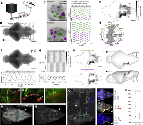
Brain responses to unilateral directional stimulation of neuromasts (A) Stimulation and acquisition setup including two-photon laser scanning microscope (2p LSM), and the stimulation capillary. (B) Maximal z-projection of the reference brain with the region that was imaged boxed in blue. Orange box shows the location of the PLLG ipsilateral to the stimulation side. MON – Medial Octavolateralis Nucleus. A – anterior, L – left, R – right, P – posterior. (C) Activity of individual pLANs in the PLLG ipsilateral to the stimulation side in two larvæ before and after whole-brain scanning. Green and magenta colors show location of responsive cr and rc pLANs, respectively. Traces show z-scored fluorescence of respective pLANs averaged across planes. Note that after whole-brain scanning, the responses of pLANs to stimulation remained similar to the initial responses. (D) Location of all responsive ROIs. Black arrowhead indicates that there were no responsive ROIs in the contralateral PLLG. (E) Bimodal distribution of the phase of the power spectrum frequency component corresponding to the stimulation frequency (see Methods for details). (F) Two example cr- and rc-selective ROIs. (G) Activity of all cr- and rc-selective ROIs detected in all imaged larvæ. The bottom image shows activity, averaged across animals; shaded areas denote SEM across larvæ. (H) Location of all cr- and rc-selective ROIs in the reference brain. Color map is the same as in D. (I) Anatomical regions of the reference brain that contained cr- and rc-selective ROIs consistently across larvæ. (J and K) A maximal projection confocal image of a Gad1b-EGFP (green) ; Sill:Cherry (red) double transgenic fish at 6dpf (dorsal view in J and lateral view in K) showing the relative position of the LAN central lintel (dashed areas). Midbrain-hindbrain boundary is shown by a vertical dashed white line, and PLL ganglion by a white arrow. (L) A magnification of a portion of the LAN central projections (red) and Gad1b(+) neurons (green), showing spatial proximity. (M) Snapshot of a dorsal view of a larval zebrafish reference brain, taken from the mapZebrain Atlas database, depicting all available single-neuron traces. Dashed area indicates the position of the LAN central lintel and white arrow the position of the PLLG. (N) Same reference brain with 3 Gad1(+) neurons overlaid, colored green (ref. 12387), blue (ref. 12352) and red (ref. 12344) in the mapZebrain Atlas. The white dot is an arbitrary spatial reference used to evaluate neuronal projection is three-dimensional renderings (not shown). (O) Magnification of the neurons shown in (N). All 3 Gad1(+) neurons project contralaterally within the hindbrain. (P) Reference brain (gray) overlaid with Gad1(+) neurons. (Q) Reference brain (gray) overlaid with functional cr an rc maps (respectively, green and red). White arrowhead indicates the posterior lateralis ganglion ipsilateral to the mechanical-stimulated side of the fish. Note lack of calcium signal on the contralateral ganglion. (R) Gad1b stack overlaid with functional cr an rc maps (respectively, in green and red, whose overlap is yellow). (S) The number of active voxels overlapping with the Gad1b binary mask. Each fish contributes one point to each category in the x axis, the horizontal line denotes the mean number of voxels across fish and the vertical line denotes the standard deviation. p value = 0.0281 (Mann-Whitney-U-Test). Scale bars are 100 μm in (A) –(I) and 50 μm in (J) –(R). See also Figure S4.

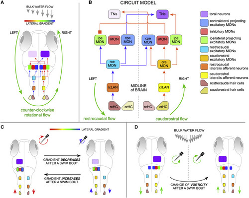
Model circuit of rheotaxis (A) Two-dimensional scheme of the model circuit represented within a larval zebrafish. Rotational flow (counter-clockwise) is represented by green circular arrows. A gradient of flow velocity is represented as a rainbow bar assigning the highest water-velocity gradient in red, and the lowest in blue). Here, only the positively stimulated HCs and LANs are shown. (B) The model circuit with transmission of rostrocaudal flow (repreesented as blue arrows within) and causdostral flow (red arrows within). Inter-hemispheric activity differences upon rotational flow and cross-hemispheric inhibition break symmetry of the system and solve vectorial ambiguity. Acronyms are spelled out on the right. (C) Top view of larval zebrafish performing rheotaxis under laminar water flow. A gradient of flow velocity is represented as a rainbow bar. As the fish swims in bouts across the horizontal plane, it will experience a decrease (red-to-blue transition) or increase (blue-to-red transition) in the magnitude of the rotational flow, which is directly linked to the gradient of bulk water flow. If gradient increases or decreases, the neuronal activity in the TNs will change (intensity differences in lilac) regardless of vorticity handedness. For simplicity, and because the system is lateral symmetric, only the active cells are depicted. (D) If the direction of rotation of local flow reverses when animals cross the midline of the water column (or experiences reversal of rotation flow upon its own directional changes across the horizontal plane), the system would simply undergo a mirror symmetric reversal of information reaching the brain. See also Figure S5.