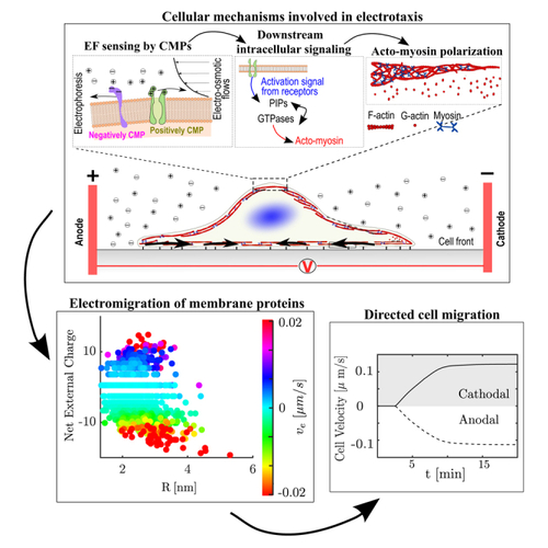
Mechanisms and model description (A) Sketch of the main processes involved in electrotaxis. Left box: Two competing forces polarize charged cell membrane components. First, an EF exerts forces on the net electric charge of the cell membrane, pulling it in a certain direction (electrophoresis). The generation of an electroosmotic flow by the EF that transports soluble ions and fluid outside the cell (electroosmosis) also generates drag forces on the membrane proteins. Middle box: The polarization of membrane components induces intracellular signals involved in the cell polarization of the actomyosin network that controls the direction of migration (right box). (B) A 1D electrotaxis model couples CMPs polarization, intracellular signals, and gel active models (see STAR Methods for details on the description of model variables and governing equations) to establish the cell migration velocity (direction and magnitude). The retrograde flow, , (black arrows) moves from the cathodal and anodal cell front inwards (sub-indexes c and a in the variables, respectively). The polymerization velocity (, blue arrow) points outwards from the cell membrane. The position of the apical side of the cell is denoted by and the one facing the cathodal one is denoted by .

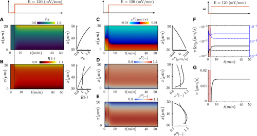
Computational results of a cell stimulated with an EF of 120 mV/mm with -potential difference of 50.76 (A–E) Kymograph of model variables along the initial cell length (Y axis) over time (X axis): CMPs polarization (A), intracellular signals (B), retrograde flow (C), actin (D), and myosin (E) densities. At the right of each panel, the CMPs, the intracellular signals (responder, solid line, and activator, dash line), the retrograde flow, actin (F-actin, solid line, G-actin, dash line) and myosin densities (bound, solid line, unbound, dash line) are shown at steady state; Retrograde flow (solid), blue and black at the cathodal and anodal sides of the cell, respectively, and polymerization velocity (dash), black and blue at the cathodal and anodal sides of the cell, respectively (F); Migration velocity of the cell (G). Color bars are differentiated by transmembrane, internal signal and actomyosin network variables.

Effect of an electric field in CMPs Color map of the model results for (A) electromotility and (B) migration velocities. The results are computed for a -potential difference in a range of −60 to 60 and an EF stimulus in a range of 50–500 . (C) Results of electromigration velocities on transmembrane proteins when electroosmosis and electrophoresis are active and (D) when electroosmotic flows have been canceled. (E and F) For those proteins that electromigrate toward the cathode and the anode, we compute the PDF for the control (electro-osmosis + electrophoresis) and the modified system (only electrophoresis). The PDFs have been normalized by using multivariable analysis, meaning that the sum of the areas for the two distributions adds to 1—this helps visualize which case dominates in that particular velocity regime.

Effect of the CMPs polarization in the signaling network and migration of the cell (A) Schematic representation of the signaling interactions. Arrows indicate positive feedback (activation) from one component to another. Tails indicate negative feedback (inactivation) of one component by another. and are the magnitudes of feedback for activating Cdc42 and Rac1 by PIP3. are the strength of the signal from receptors to GTPases or PI3K. (B–F) Two cases are shown, where the gradient of receptors that activates PI3K is always polarized toward the cathode (gray gradient) and the polarization of receptors that activate Rac1 and Cdc42 are toward the cathode (B and E) or the anode (C and F). (B and C) Evolution in time of Rac (blue), Cdc42 (red) and Rho (black), and PIPs (E and F) in the cathodal (dash) and anodal (solid) side of the cell are presented. (D) Cell migration velocity for the cases presented in (B–E) and (C–F). For the case presented in (B and C), we vary the strength of the stimulus , , and in a normal feedback loop from PIP3 to Cdc42 and Rac1 (G), when no feedback loop to Cdc42 (H) and no feedback loop to Rac1 (I). For the three cases presented in (G) in points (J–L) we vary the strength of the feedback loop from PIP3 to Cdc42 and Rac1.