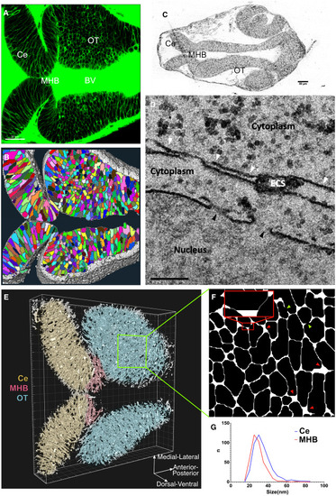
The in silico architechture of zebrafish brain atlas. (A) Expression of sec-EGFP in zebrafish brain at 24 hpf (scalebar, m). (B) Segmentation of cells (color coded) and ECS (white) from 3D fluorescent image stack (materials and methods). (C) Brightfield image of thick section (thickness, 500 nm) of brain slice to provide location reference of different brain regions for following EM acquisitions (scalebar, 50 ?m). (D) TEM image captured ECS from Ce region and nuclear pore as reference. White arrowheads indicate ECS, with width measurements: 31, 22, 26, and 85 nm from left to right. Black arrowheads indicate nuclear pores, and the diameters are 91 and 110 nm from left to right (scalebar, 200 nm). (E) 3D in silico representation of the brain atlas of 24-hpf zebrafish. (F) Zoomed-in slice from the OT region, showing the voids (red arrowheads) and ECS channels (red insertion) in 2D. The inset highlights two narrow ECS channels with 20 nm width separated by a void. Green arrowheads indicate dead ends. (G) Distribution of ECS widths from Ce and MHB region. The overall width of the ECS lies in the range 15?85 nm. The widths of ECSs measured were nm (mean SD) in OT and MHB and nm in Ce.

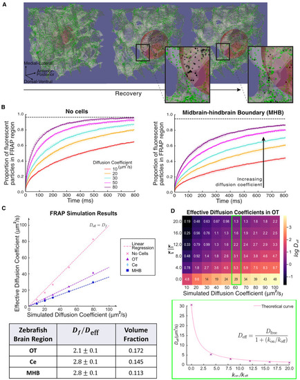
In silico FRAP simulations. (A) Example outputs of simulated FRAP measurements in the OT of the zebrafish brain, represented by the white translucent skeleton. Green and black dots represent discrete fluorescent and photobleached molecules, respectively. Red sphere represents photobleached region of radius 6 ?m. The second and third panels are zoomed in by a factor of two compared to left hand panel, to better visualize the FRAP region during recovery. The insets show a close-up of particles diffusing in a tortuous environment, showing the distribution of bleached and fluorescent particles before and after recovery. (B) Recovery curves for molecules with input ?m2/s for simulations without cells and midbrain-hindbrain boundary environments (solid lines and shaded regions represent the mean and standard deviations of simulated experiments, respectively). The curves are generated from 10 experiments consisting of simulating 20,000 independent particles in parallel. Each simulation is fitted with Soumpasis diffusion (Eq. (5)) (dashed lines) to obtain average diffusion time constant, . Black horizontal dashed lines represent the maximum intensity, the recovery curve will converge to since the system is conserved. (C) Results of the measured effective diffusion coefficients, , for different regions in the zebrafish brain obtained from recovery curves such as in (B). The table shows the average factor decrease in effective diffusion coefficient, which is the reciprocal of the gradients of the fitted dashed lines. Volume fraction indicates the proportion of the ECS volume to the volume of the full tissue segment. (D) Heatmap of the effects of transient binding. Values indicate the measured using the same technique, for different values of and input diffusion coefficient . The Color of the heatmap is on log scale. Lower panel shows as a function of , with simulation results (crosses) and theoretical curve (solid line).

In silico FCS simulations. (A) Binary image shows a slice of the OT region marked with examples of a void and channel detection region for FCS experiments by red circles. Detection region is a sphere of radius 0.1 ?m. On the right is shown an example output of the "intensity" profile by counting the number of particles in the detection region at each simulation time step, which is 0.04 ms. The black dashed line is the mean number of particles across the simulation related to in the autocorrelation plots. (B) FCS experiments simulated for different regions (void and channels) of OT images for the cases without binding (left) and receptor bindings on cell surfaces (right). Mean temporal autocorrelation (solid and dashed lines) with standard deviation (shaded regions) of the "intensity" profiles for increasing lag times is plotted on a log scale and fitted with 3D diffusion model (Eq. (9)). Left figure shows autocorrelation curves of different colors for diffusion coefficients 10?80 ?m2/s for voids (solid lines) and channels (dashed lines) without binding events. Linear regression (inset) shows that measured approximately recovers the input diffusion coefficient in this parameter regime, with channel region showing slightly more slowdown due to hindered diffusion. The right figure shows mean autocorrelation curves for voids and channels with receptor bindings at cell surfaces. This shows two populations, slow- and fast-diffusing molecules in the system, localized in the channel and void regions, respectively. For FCS in voids (purple), the measured is m2/s, whereas FCS data in channels were fitted with a two-species model, in which of particles were a slow-diffusing component with fitted m2/s. (C) FCS experiment is simulated in voids for different architectures of the zebrafish brain for ?m2/s, and curves for ?m2/s for simulation on different architectures are shown here. measurements are of similar magnitude as the input diffusion coefficient , showing that FCS measurements recover the input diffusion coefficient of the simulations. This shows that surrounding tortuosity does not affect results when measuring local diffusion coefficient.

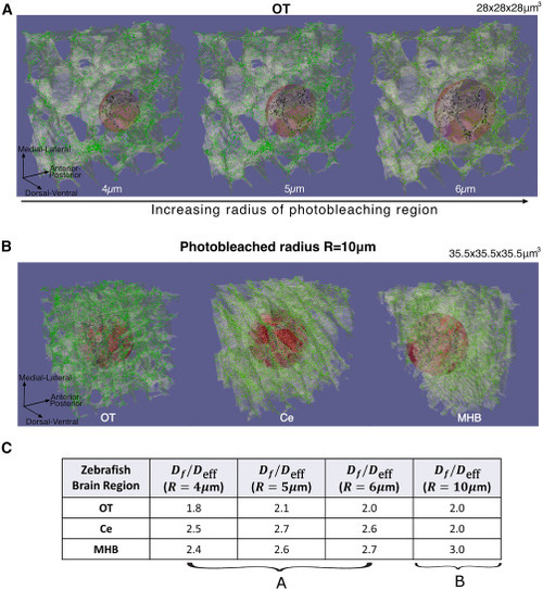
FRAP simulations on different photobleaching radius sizes. (A) Simulations of FRAP with photobleaching regions of spheres with different radius sizes, ?m (left to right). ?m3 tissue segments were used for FRAP simulations. (B) Full 3D image of FRAP on OT, Ce, and MHB regions (left to right), where the photobleaching region was ?m. ?m3 tissue segments were used for these sizes of FRAP simulation. This shows that the tissue structure varies across zebrafish brain regions. (C) Values of from FRAP experiments for the various radius sizes, showing that we obtain a factor of around 2?3 decrease of effective diffusion coefficient for various zebrafish brain regions. The values show that FRAP results may slightly vary depending on the tissue architecture surrounding the photobleached region.

FRAP simulations with varying image connectivity. (A) OT images with altered dead-end percentage. (B) Results from FRAP experiments by simulating the particle model on OT images with dead ends of varying volume fraction ? and dead ends. (C) with altering volume fraction, ?, for different environments and varying connectivity. The green box highlights that adding dead ends reduced the diffusion coefficient more drastically than reducing volume fraction of connected spaces. Here, the altered OT images with dead ends were dilated across the entire stack so that ? was kept relatively similar to the connected OT image.