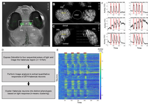
The habenula has multiple subtypes of cells that show differential response to light. (A) Dorsal view of the head of a live 7-day-old fish, with GCaMP3 expression in the habenula (arrows) under the control of the s1011t GAL4 driver. (B) A single two-photon slice through the dorsal habenula of the fish in panel A (boxed region). (C) A yz-reconstruction at the point indicated by the yellow line in panel B, showing a transverse view of the habenula. The dotted lines indicate imaging planes separated by 10 μm. The yellow line indicates the plane imaged in B. Dashed lines show the border of the habenula. (D) Workflow of habenula analysis (E) Heat map showing the activity of 2974 individual neurons (rows) across multiple light on and off cycles. Red bars on top correspond to the time period when light is switched on. As seen, some neurons show higher activity during light exposure (ON cells) and some neurons show higher activity after the light is switched off (OFF cells). (F) Response (y-axis) vs. time (x-axis) for habenula neurons that were clustered into subgroups depending on their response to light. Pink regions in each plot corresponds to the light exposure period. Seen here are the three subtypes in the dorsal habenula region (left) and three in the ventral habenula region (right). In total six subtypes were identified: D-ON-Tonic, D-OFF-Tonic, D-OFF-Phasic, V-ON-Tonic, V-OFF-Tonic, and V-OFF-Phasic. lHb: left habenula; rHb: right habenula; a: anterior; p: posterior. Scale bar = 25 μm

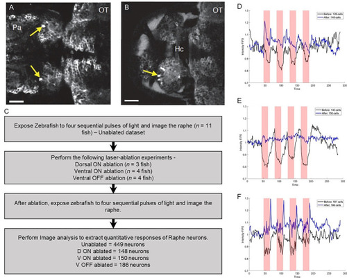
The effects of lesioning specific cells in the habenula on raphe response to irradiance change. (A-B) Examples of lesioning. The arrows indicate individual cells with elevated levels of intracellular calcium, following two-photon laser lesioning. (C) Workflow of raphe analysis. (D-F) The response of raphe (y-axis) vs. time (x-axis) when the habenula is intact (black curve) vs. when specific cells are lesioned in the habenula (blue curve). Red regions correspond to periods of light exposure. When the habenula is intact, the raphe is inhibited during light exposure in all three experiments. (D) The raphe shows inconsistent activation during light exposure when ON cells in the dorsal habenula (D-ON) are ablated. (E) The raphe is almost unresponsive when ON cells in the ventral habenula (V-ON) are ablated. (F) The raphe shows activation as soon as light is switched off, when the OFF cells in the ventral habenula (V-OFF) are ablated

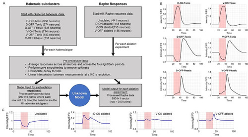
Characteristic responses of habenula and raphe to one light-dark cycle. (A) Schematic showing the workflow and data structures obtained from processing the raw neuronal activity data from the habenula and the Raphe. The “Unknown Model” represents an as-yet unknown model whose goal would be to use the habenula data as input to estimate raphe behaviour from the ablation experiments. (B) Characteristic responses of the six habenula subtypes to light exposure were obtained by averaging across the four light-dark periods. This was followed by padding and interpolation to extend the response trajectory to 100s so all neurons would reach the baseline, followed by smoothing. (C) Characteristic responses of raphe neurons to unablated conditions or ablation experiments were obtained from the response of individual raphe cells to the first light exposure and following dark period

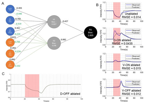
Neural network model and estimated raphe behavior. (A) The final neural network model that was able to recapitulate raphe behaviour from habenula input. The first layer of the network has six nodes corresponding to the six habenula subtypes. The middle layer has two nodes and the final output layer has one node whose output is the estimated raphe behaviour. The numbers on the edges represent the weights of the edge. (B) Observed raphe behaviour (blue) and model-estimated raphe behaviour (dotted gray) for the unablated and the ablation experiments shows good fit (RMSE of the fit shown on the plots) (C) Model-estimated raphe response for a potential D-OFF ablation experiment

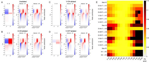
Contributions of each neural network node to the Raphe response. (A-D) Contributions (y-axis) of each NN node (x-axis) to the nodes in the successive layer over 100s (y-axis). In each panel, the leftmost column shows the contribution of H1 and H2 nodes to the Raphe output (after scaling by the respective Layer 2 weights). The middle panel shows the contribution of the six Habenula subtypes to the H1 node (after scaling by the respective Layer 1 weights), and the right most column shows the contribution of the same six habenula subtypes to the H2 node (after scaling by the respective Layer 1 weights). The contribution intensities are indicated by the color scheme ranging from negative/inhibition (blue) to positive/activation (red). (A) shows the node contributions in the unablated experiment, (B) in the D-ON ablation experiment, (C) in the V-ON ablated experiment and (D) in the V-OFF ablation experiment. In the ablation experiments, the contributions of the ablated neurons can be seen to be zero. (E) shows the sensitivity of the final estimated Raphe output to changes in each NN parameter. The intensities show the fit error computed as the RMSD between the model-estimated and observed Raphe responses across the unablated and three ablation experiments