
- Title
-
Optimised tissue clearing minimises distortion and destruction during tissue delipidation
- Authors
- Lee, K., Lai, H.M., Soerensen, M.H., Hui, E.S., Ma, V.W., Cho, W.C., Ho, Y.S., Chang, R.C.
- Source
- Full text @ Neuropathol. Appl. Neurobiol.
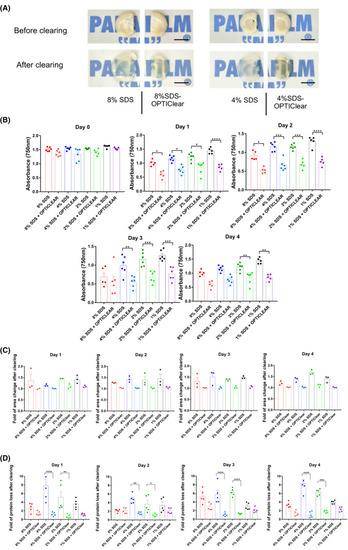
Tissue clearing with different concentrations of SDS vs SDS‐OPTIClear. (A) Representative images of 4 mm‐thick rat brain tissues before and after clearing with SDS and SDS‐OPTIClear respectively. Scale bar = 5 mm. (B) Absorbance at 750 nm for tissues cleared at varying concentrations of SDS vs SDS‐OPTIClear (n = 5–6). Lower absorbance level indicates higher transparency level. (C) Fold of area change after clearing with SDS compared to SDS‐OPTIClear (n = 3). Tissue sizes were quantified and normalised to the size of tissue before clearing. (D) Fold of protein loss after clearing for SDS only compared to SDS‐OPTIClear (n = 5–6). Solutions used for clearing were collected and then added to a stain‐free gel for electrophoresis, band intensities were quantified and normalised with the protein band intensity of sample solution collected at day 0 (before clearing). Mean ± SEM for all graphs. Two‐way ANOVA, Tukey's multiple comparison test, *p ≤ 0.05, **p ≤ 0.01, ***p ≤ 0.001, ****p ≤ 0.0001 |

Tissue distortion level after clearing with different conditions. 1 mm‐thick rat tissues were stained with TO‐PRO®‐3 and then imaged before delipidation, after delipidation and after RI‐matching in OPTIClear. (A) Representative images of TO‐PRO®‐3 stained tissues under different stages of clearing. White dotted lines marked the original boundary of tissues. Scale bars = 1 mm (n = 3). (B) Fold tissue area changes after tissue clearing and RI‐matching, respectively. (C) Percentage changes in dorsal–ventral (D‐V) and mediolateral (M‐L) lengths after RI‐matching respectively (n = 3). (D) Percentage changes in the ratio of D‐V and M‐L length after RI‐matching (n = 3). (E) Merged images of GFP‐labelled hippocampal neurons under different stages of clearing. The same neuron was imaged before and after clearing, and after RI‐matching. Images were labelled with different colours (see Fig. S3 and merged together. Higher degree of overlapping indicates lower distortion level in morphology. Scale bars = 20 µm. Mean ±S.E.M. for all graphs. Two‐way ANOVA, Tukey's multiple comparison test, *p ≤ 0.05, **p ≤ 0.01, ***p ≤ 0.001, ****p ≤ 0.0001 |

Comparison between 3D immunostaining of tissue cleared with SDS and SDS‐OPTIClear. (A) Iba‐1 staining of tissues cleared with 4% SDS‐OPTIClear (left panel) and 4% SDS only (right panel). Upper panel: images taken with a 10× objective. Lower panel: zoomed‐in image of the dentate gyrus (DG) taken with a 20× objective (left image), Z‐stack images taken with a 63× objective with z‐depth = 161.7 μm (right image). (B) TOMM‐20 staining of regions cleared with 4% SDS‐OPTIClear (left panel) and 4% SDS only (right panel). Left image: 20× images of DG regions. Right image: z‐stack of the images showed on the left (z‐depth = 125.84 μm). (C) ChAT staining taken with a 20× objective. Left panel: 20× images of the nbM cleared with 4% SDS and 4% SDS‐OPTIClear. Right panel: z‐stack of the images showed in the left panel (z‐depth = 72 μm). The same imaging and display settings were used for both 4% SDS and 4% SDS with OPTIClear conditions |
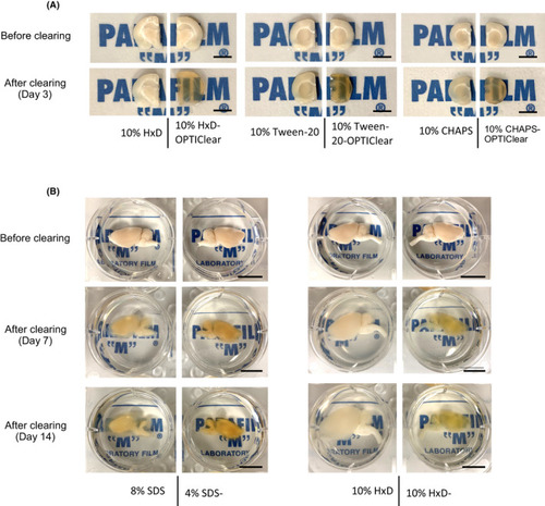
Comparison of clearing efficiency between combinations of OPTIClear with different detergents. (A) Representative images of tissues before and after clearing (scale bar = 5 mm) (B) Comparison of clearing efficiency between combinations of OPTIClear with SDS and 1,2‐Hexandiol (HxD). Representative images of rat brain hemispheres before and after clearing were shown. (scale bar = 10 mm) |
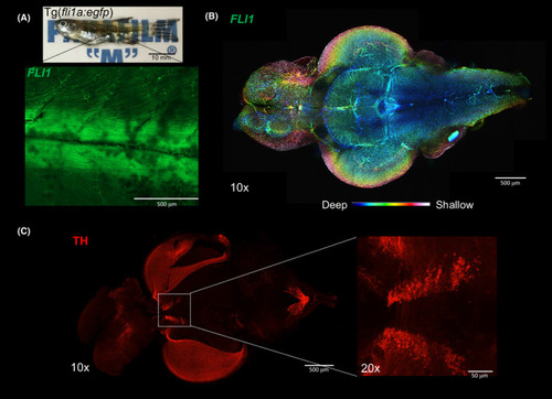
Zebrafish (Danio rerio) imaging after tissue clearing. (A) Whole Tg(fli1a:EGFP) y1 (1.5 years old) after clearing with 4% SDS‐OPTIClear, scale bar = 10 mm. Zoomed‐in 10× image showing EGFP fluorescence in blood vessels. (B)Colour‐coded image labelling the blood vessels in whole zebrafish brain, scale bar = 500 μm. (C) Whole brain immunostained with antibodies against tyrosine hydroxylase, scale bar = 500 μm, higher magnification (20×) showing posterior tuberculum, scale bar = 50 μm |
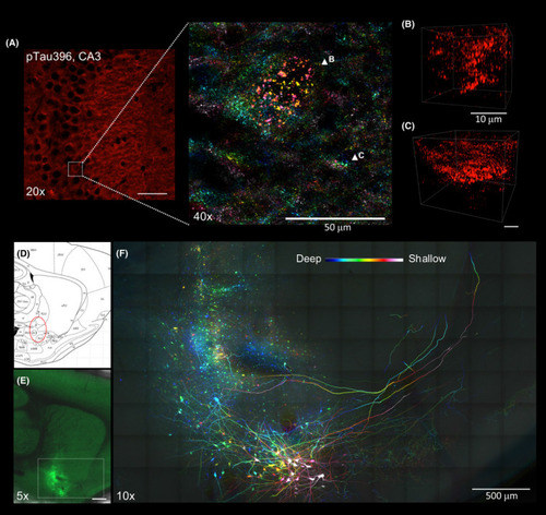
Applications of Accu‐OptiClearing in rodent brain tissues. Visualisation of phosphorylated tau aggregation in 3xTg mice. (A) Image of the hippocampal CA3 region stained with anti‐phosphorylated tau antibody. Inset showing colour‐coded projection of phosphorylated tau‐positive aggregations (indicated by arrowheads in B and C). Scale bar, 50 μm (for A), 10 μm (for B and C). Long‐range tracing of rat nucleus basalis of Meynert neurons with AAV‐GFP. (D) Sagittal rat brain atlas indicating the nbM region in red dotted circle. (E) Tiled Z‐stack image showing AAV‐GFP‐labelled nbM neurons three weeks after injection into the nbM region (scale bar = 1 mm). (F)Colour‐coded projection image with higher magnification of the region shown in E (scale bar = 500 μm, z‐depth = 205 μm) |