ZFIN All Figures, Song <i>et al.</i>, 2021

Figure 1.

Positional information transfer by the morphogen gradient.

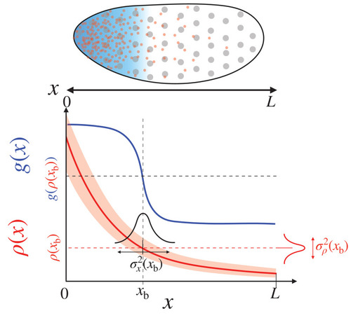
(Top) The specification of the anterior region of the fruit fly embryo. The uniformly distributed nuclei (gray circles) are subjected to different concentrations of the morphogen (red dots) in the local environment, which leads to the anterior expression of the target gene (blue shade). (Bottom) The red and blue lines respectively depict the morphogen profile, $ρ (x)$ $ρ (x)$ , and the target gene expression, $g (x)$ $g (x)$ , which together specify cell fate. The squared positional error at the boundary $x_{b}$ $x_{b}$ , $σ_{x}^{2} (x_{b})$ $σ_{x}^{2} (x_{b})$ , is defined as the product between the variance of the morphogen concentration, $σ_{ρ}^{2} (x_{b})$ $σ_{ρ}^{2} (x_{b})$ , and the squared inverse slope of the morphogen profile, ${(\partial_{x} ρ (x))}_{x = x_{b}}^{- 2}$ ${(\partial_{x} ρ (x))}_{x = x_{b}}^{- 2}$ .

Figure 2

Cost-precision trade-off associated with the point measurement.

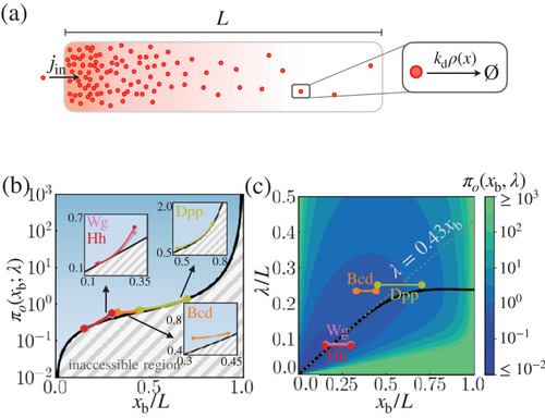
(a) Schematic of the model. (b) The position-dependent lower bound of the trade-off product $π_{o, \min} (x_{b})$ $π_{o, \min} (x_{b})$ , obtained numerically. The gray hashed area represent the inaccessible regions. The trade-off product of the morphogen profiles of Bcd, Wg, Hh, and Dpp are shown in the respective insets. (c) The black line denotes the optimal characteristic decay length ( $λ_{\min}$ $λ_{\min}$ ) with respect to the position $x_{b} / L$ $x_{b} / L$ . The color scale indicates the trade-off product $π_{o} (x_{b})$ $π_{o} (x_{b})$ computed for each pair of $λ / L$ $λ / L$ and $x_{b} / L$ $x_{b} / L$ values. The grea dotted line depicts the linear approximation of $λ_{\min}$ $λ_{\min}$ at large $L$ $L$ . In (b) and (c), the depicted trade-off product is normalized by $α_{o} L / l_{cell}$ $α_{o} L / l_{cell}$ . The parameters for the naturally occurring morphogen profiles are further described in Appendix 3, Length scales of Bcd, Wg, Hh, and Dpp, and Appendix 3—table 1.

Figure 3.

Cost-precision trade-off associated with the space-time-averaged measurement.

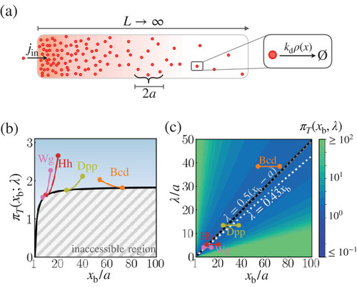
(a) Schematic of the model. (b) The optimal trade-off product $π_{T} (x_{b})$ $π_{T} (x_{b})$ obtained numerically with respect to the location of the target boundary position normalized by the sensor size ( $x_{b} / a$ $x_{b} / a$ ). The gray hashed area represent the inaccessible regions. Shown are the trade-off products of the morphogens profiles of Bcd, Wg, Hh, and Dpp. (c) The black line denotes the optimal characteristic decay length ( $λ_{\min}$ $λ_{\min}$ ) with respect to the position $x_{b} / a$ $x_{b} / a$ . The color scale indicates the trade-off product $π_{T} (x_{b})$ $π_{T} (x_{b})$ computed for each pair of $λ / a$ $λ / a$ and $x_{b} / a$ $x_{b} / a$ values. The gray dotted line depicts the linear approximation of $λ_{\min}$ $λ_{\min}$ . The white dotted line depicts the linear approximation of $λ_{\min}$ $λ_{\min}$ for the point measurement model. In (b) and (c), the depicted trade-off product is normalized by $α_{o}$ $α_{o}$ . The parameters for the naturally occurring morphogen profiles are further described in the Appendix 3, Length scales of Bcd, Wg, Hh, and Dpp, and Appendix 3—table 1.

Figure 4.

Optimal concentration profile of morphogens.

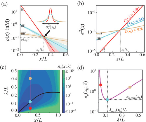
(a) Three possible morphogen profiles (i) (red), (ii) (cyan), (iii) (brown) with different λ’s ( $λ^{(i)} < λ^{(i i)} < λ^{(i i i)}$ $λ^{(i)} < λ^{(i i)} < λ^{(i i i)}$ ), generated with different values of morphogen influxes $j_{i n}$ $j_{i n}$ ( $j_{in}^{(i)} > j_{in}^{(ii)} > j_{in}^{(iii)}$ $j_{in}^{(i)} > j_{in}^{(ii)} > j_{in}^{(iii)}$ ). The morphogen concentration of the three profiles coincide at $x_{b}$ $x_{b}$ , giving rise to the same threshold value $ρ (x_{b})$ $ρ (x_{b})$ but different positional errors ( $ϵ^{2} (x_{b}; λ)$ $ϵ^{2} (x_{b}; λ)$ ). (b) The precision of three possible morphogen profiles (i) (red), (ii) (cyan), (iii) (brown) with different λ’s ( $λ^{(i)} < λ^{(i i)} < λ^{(i i i)}$ $λ^{(i)} < λ^{(i i)} < λ^{(i i i)}$ ), generated with different values of morphogen influxes $j_{i n}$ $j_{i n}$ ( $j_{in}^{(i)} > j_{in}^{(iii)} > j_{in}^{(ii)}$ $j_{in}^{(i)} > j_{in}^{(iii)} > j_{in}^{(ii)}$ ). The λ values are identical to those with matching colors in (a), but the red and brown curves are generated with different $j_{i n}$ $j_{i n}$ values from those in (a). The cost associated with each morphogen profile are shown in units of $α_{o} L / l_{cell}$ $α_{o} L / l_{cell}$ . (c) The diagram of the trade-off product associated with the point measurement, $π_{o} (x; λ)$ $π_{o} (x; λ)$ , plotted with respect to $x$ $x$ and λ. The black line indicates the optimal decay length, $λ_{\min}$ $λ_{\min}$ at position $x$ $x$ . Shown on the diagram are the trade-off product $π_{o}$ $π_{o}$ ’s for the three cases shown in (a) and (b). (d) The value of $π_{o}$ $π_{o}$ as a function of λ at $x = x_{b}$ $x = x_{b}$ . The trade-off product is minimized to $π_{o} = π_{o}^{(ii)} \approx α_{o} (L / l_{cell}) 0.4$ $π_{o} = π_{o}^{(ii)} \approx α_{o} (L / l_{cell}) 0.4$ with $π_{o}^{(ii)} < π_{o}^{(iii)} < π_{o}^{(i)}$ $π_{o}^{(ii)} < π_{o}^{(iii)} < π_{o}^{(i)}$ .

Acknowledgments

This image is the copyrighted work of the attributed author or publisher, and ZFIN has permission only to display this image to its users. Additional permissions should be obtained from the applicable author or publisher of the image. Full text @ Elife

Song et al., 2021

ZDB-PUB-210923-2
PMID:34402427

Cost-precision trade-off relation determines the optimal morphogen gradient for accurate biological pattern formation

Positional information transfer by the morphogen gradient.

Cost-precision trade-off associated with the point measurement.

Cost-precision trade-off associated with the space-time-averaged measurement.

Optimal concentration profile of morphogens.

Song et al., 2021 ZDB-PUB-210923-2 PMID:34402427

Cost-precision trade-off relation determines the optimal morphogen gradient for accurate biological pattern formation

Positional information transfer by the morphogen gradient.

Cost-precision trade-off associated with the point measurement.

Cost-precision trade-off associated with the space-time-averaged measurement.

Optimal concentration profile of morphogens.

Song et al., 2021

ZDB-PUB-210923-2
PMID:34402427