ZFIN Image: Song et al., 2021, Figure 4.

Image

Figure Caption

Figure 4.

Optimal concentration profile of morphogens.

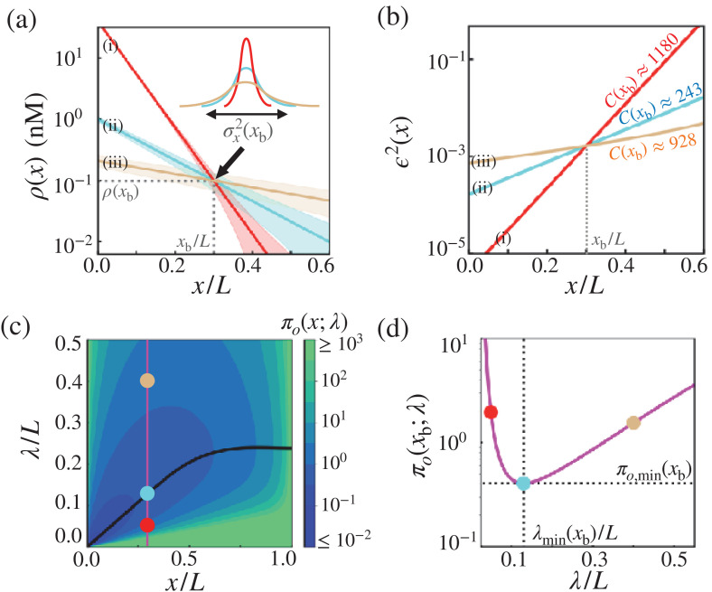
(a) Three possible morphogen profiles (i) (red), (ii) (cyan), (iii) (brown) with different λ’s ( $λ^{(i)} < λ^{(i i)} < λ^{(i i i)}$ $λ^{(i)} < λ^{(i i)} < λ^{(i i i)}$ ), generated with different values of morphogen influxes $j_{i n}$ $j_{i n}$ ( $j_{in}^{(i)} > j_{in}^{(ii)} > j_{in}^{(iii)}$ $j_{in}^{(i)} > j_{in}^{(ii)} > j_{in}^{(iii)}$ ). The morphogen concentration of the three profiles coincide at $x_{b}$ $x_{b}$ , giving rise to the same threshold value $ρ (x_{b})$ $ρ (x_{b})$ but different positional errors ( $ϵ^{2} (x_{b}; λ)$ $ϵ^{2} (x_{b}; λ)$ ). (b) The precision of three possible morphogen profiles (i) (red), (ii) (cyan), (iii) (brown) with different λ’s ( $λ^{(i)} < λ^{(i i)} < λ^{(i i i)}$ $λ^{(i)} < λ^{(i i)} < λ^{(i i i)}$ ), generated with different values of morphogen influxes $j_{i n}$ $j_{i n}$ ( $j_{in}^{(i)} > j_{in}^{(iii)} > j_{in}^{(ii)}$ $j_{in}^{(i)} > j_{in}^{(iii)} > j_{in}^{(ii)}$ ). The λ values are identical to those with matching colors in (a), but the red and brown curves are generated with different $j_{i n}$ $j_{i n}$ values from those in (a). The cost associated with each morphogen profile are shown in units of $α_{o} L / l_{cell}$ $α_{o} L / l_{cell}$ . (c) The diagram of the trade-off product associated with the point measurement, $π_{o} (x; λ)$ $π_{o} (x; λ)$ , plotted with respect to $x$ $x$ and λ. The black line indicates the optimal decay length, $λ_{\min}$ $λ_{\min}$ at position $x$ $x$ . Shown on the diagram are the trade-off product $π_{o}$ $π_{o}$ ’s for the three cases shown in (a) and (b). (d) The value of $π_{o}$ $π_{o}$ as a function of λ at $x = x_{b}$ $x = x_{b}$ . The trade-off product is minimized to $π_{o} = π_{o}^{(ii)} \approx α_{o} (L / l_{cell}) 0.4$ $π_{o} = π_{o}^{(ii)} \approx α_{o} (L / l_{cell}) 0.4$ with $π_{o}^{(ii)} < π_{o}^{(iii)} < π_{o}^{(i)}$ $π_{o}^{(ii)} < π_{o}^{(iii)} < π_{o}^{(i)}$ .

Acknowledgments

This image is the copyrighted work of the attributed author or publisher, and ZFIN has permission only to display this image to its users. Additional permissions should be obtained from the applicable author or publisher of the image. Full text @ Elife