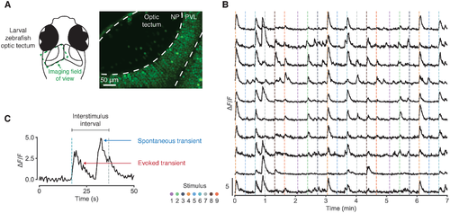
Fig 1. Spontaneous activity in calcium imaging data. (A) Two-photon calcium imaging of the larval zebrafish optic tectum. NP, neuropil; PVL, periventricular layer. (B) Fluorescence traces from 10 example neurons. Dashed vertical lines indicate stimulus onset; colour represents azimuth angle of presented stimulus. (C) Example fluorescence trace segment illustrating that spontaneous calcium transients can occur just before stimulus onset, inflating stimulus-response estimates.

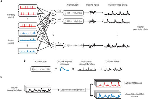
Fig 2. Overview of the CILVA approach for decoupling stimulus-evoked responses and latent sources of SA. (A) Proposed generative architecture underlying multivariate calcium imaging data. Neurons are driven by sensory stimuli (red) and latent sources of SA (blue). These two sources are combined additively to define the underlying rate of calcium influx (λn), before being convolved with a GCaMP kernel. Calcium levels are subsequently reported through noisy fluorescence intensities. (B) The intensity of calcium influx λn encoding stimuli and shared SA is convolved with a GCaMP kernel k to generate observed calcium levels. (C) The learned encoding model provides a method for decoupling evoked responses from common patterns of SA.

Fig 3. Fitted model components for the zebrafish shown in Fig 1. (A) Results of fitting CILVA and decoupling EA (red) and shared SA (blue) in an experimental recording. Inset numbers denote the Pearson correlation coefficient between raw fluorescence trace and model fit. The 10 neurons with the highest correlations between data and model fit are shown. (B) Distribution of correlation coefficients between data and model fits. Shuffled data obtained by cyclically permuting each trace by a random offset while preserving its temporal structure. (C) Inferred latent factor timeseries. Inset numbers denote the factor contribution indices, defined as the mean reduction in correlation coefficient across the population following deletion of the corresponding factor. (D) Cross-validated distributions of correlation coefficients for 1 to 15 latent factors. Shaded error bars indicate one standard deviation. For this fish adding additional latent sources of SA beyond three factors provides little improvement in the average correlation for both training and held-out test data. (E) Estimated factor coupling matrix shows that latent factors target distinct, non-overlapping sets of neurons. (F) Cumulative factor contribution indices for 0 to 3 latent factors. (G) Cross-correlograms show little interaction between latent factors and no long term structure in individual factor activity. While zebrafish can occasionally exhibit factors with secondary peaks in their autocorrelation plots (see e.g. S9H Fig), the location of these peaks varies between factors and fish, and do not align with the interstimulus interval. (H) Example estimated stimulus tuning curves (red). Tuning curves obtained by trial-averaging fluorescence levels over a window following stimulus onset (gray) provided for comparison (Methods). Shaded error bars denote one standard deviation. Full temporal traces for these neurons are given in S8 Fig. (I) Retinotopic maps obtained by trial-averaging fluorescence levels over a window following stimulus onset (left) and by CILVA-estimated tuning curves (right). The CILVA map is more refined since the estimated stimulus filters already account for ongoing SA.

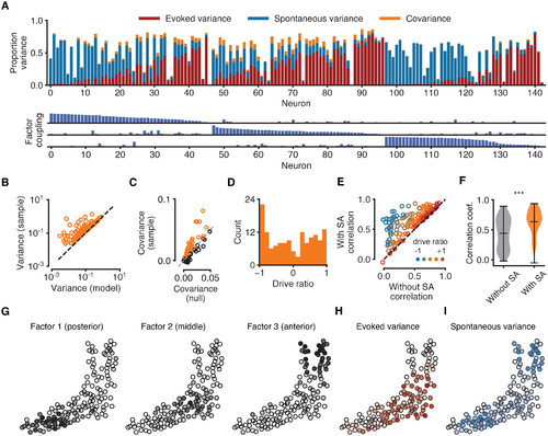
Fig 4. Analysis of the contribution of EA and SA to neural variability. All data for the same fish as in Fig 3. (A) Top: composition of each neuron’s sample variance in terms of variance attributable solely to EA (red bars), solely to shared SA (blue bars), and their covariance (orange bars). Orange bars represent absolute values of covariances for ease of visualisation. Variance components are given as proportions of the total sample variance of the raw fluorescence signal var[fn] (corrected for imaging noise, see Methods). Neurons sorted by the strength of their coupling to each factor (as in Fig 3E). Bottom: coupling between neurons and latent sources of SA suggests neurons with strong coupling are weakly driven by sensory stimuli. Maximum bar height of one. (B) Sample variance (corrected for imaging noise) vs variance of the statistical model indicates that the model does not overestimate variance. Each data point represents one neuron. (C) Covariances between evoked and spontaneous traces estimated by the model (vertical axis). Chance levels for a null model (horizontal axis) are 95th percentiles of shuffled data obtained by cyclically permuting evoked traces by random offsets 1000 times while preserving temporal structure. Sample covariances exceeding chance levels (orange circles above dashed identity line) cannot be attributed to the slow timescale of the calcium indicator. (D) Distribution of drive ratios across the population of neurons. (E) Correlation coefficient between raw fluorescence trace and evoked component of model fit (without SA) and full model fit (with SA). Neurons with strongly negative drive ratios show marked improvement in the quality of model fit. (F) Violin plots showing statistically significant improvement in the average correlation coefficient between experimental data and model fits after incorporating latent sources of SA (p < 0.001, Wilcoxon signed-rank test). (G) Spatial organisation of latent factors underlying SA. The three non-overlapping factors are spatially localised and tile the imaging plane. (H) Spatial organisation of the evoked variance components. Cell opacity is proportional to the fraction of variance attributable to EA for the given neuron. Neurons strongly driven by EA cluster in the middle region of the tectum. (I) Same as H, but for SA. Neurons strongly driven by SA cluster in the anterior and posterior tectum.

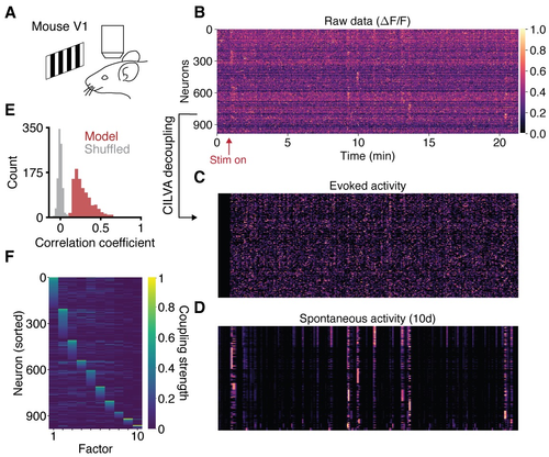
Fig 5. Single-trial decoupling of EA and SA in visual cortex. (A) Calcium imaging of mouse V1 during presentation of drifting gratings. (B) Raw data consists of 21 minutes of neural activity from 986 neurons. The fluorescence trace of each neuron is normalised to take values between 0 (dark) and 1 (light). Neurons sorted as in panel F. (C) Decoupled evoked component of neural activity. (D) Decoupled spontaneous component of neural activity, given a latent dimensionality of 10. (E) Distribution of correlation coefficients between data and model fits. Shuffled data obtained by cyclically permuting each trace by a random offset while preserving its temporal structure. (F) Learned factor coupling matrix showing that the inferred factors target largely non-overlapping sets of neurons.