Fig. 3

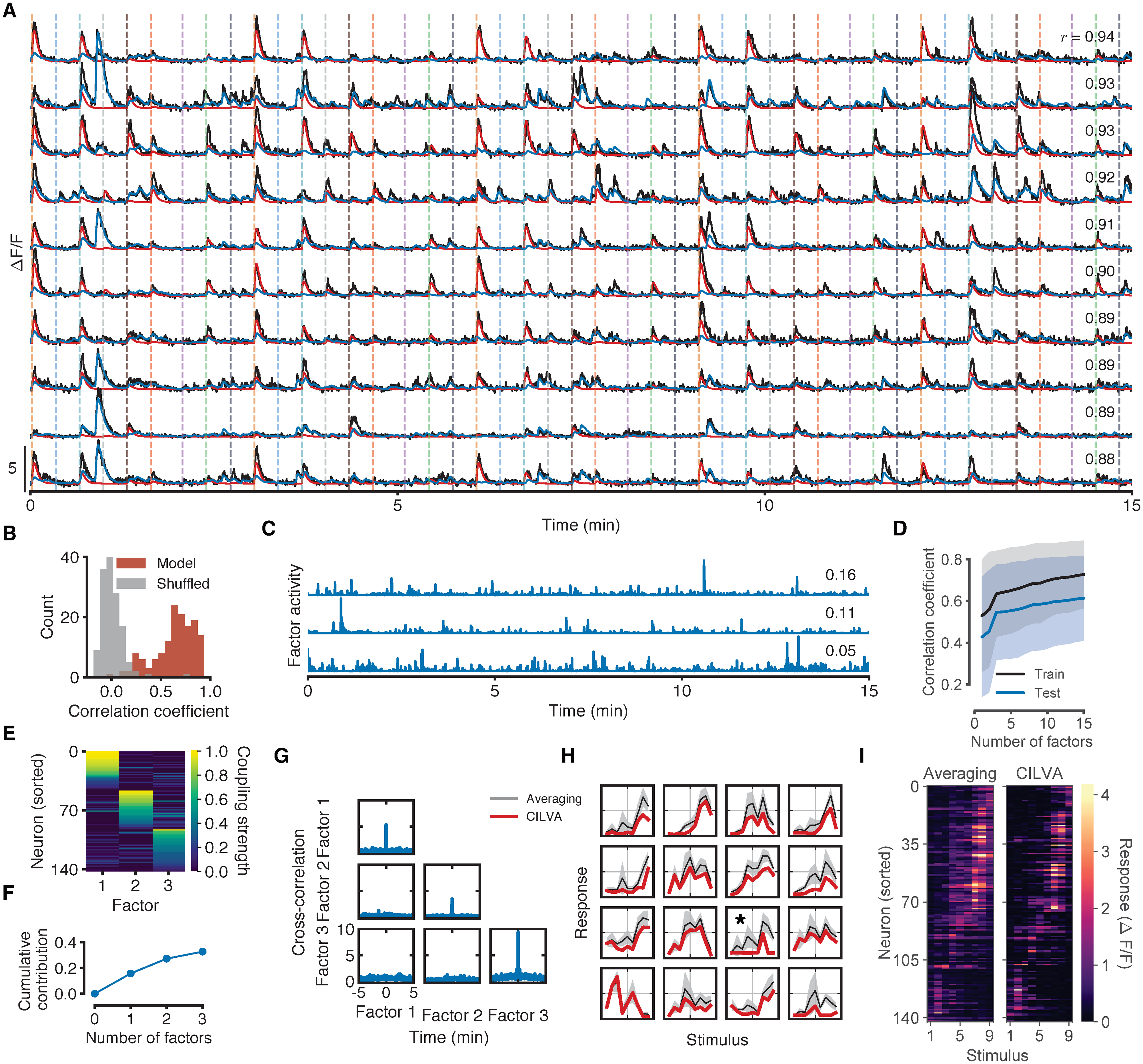
Fig. 3 Fig 3. Fitted model components for the zebrafish shown in Fig 1. (A) Results of fitting CILVA and decoupling EA (red) and shared SA (blue) in an experimental recording. Inset numbers denote the Pearson correlation coefficient between raw fluorescence trace and model fit. The 10 neurons with the highest correlations between data and model fit are shown. (B) Distribution of correlation coefficients between data and model fits. Shuffled data obtained by cyclically permuting each trace by a random offset while preserving its temporal structure. (C) Inferred latent factor timeseries. Inset numbers denote the factor contribution indices, defined as the mean reduction in correlation coefficient across the population following deletion of the corresponding factor. (D) Cross-validated distributions of correlation coefficients for 1 to 15 latent factors. Shaded error bars indicate one standard deviation. For this fish adding additional latent sources of SA beyond three factors provides little improvement in the average correlation for both training and held-out test data. (E) Estimated factor coupling matrix shows that latent factors target distinct, non-overlapping sets of neurons. (F) Cumulative factor contribution indices for 0 to 3 latent factors. (G) Cross-correlograms show little interaction between latent factors and no long term structure in individual factor activity. While zebrafish can occasionally exhibit factors with secondary peaks in their autocorrelation plots (see e.g. S9H Fig), the location of these peaks varies between factors and fish, and do not align with the interstimulus interval. (H) Example estimated stimulus tuning curves (red). Tuning curves obtained by trial-averaging fluorescence levels over a window following stimulus onset (gray) provided for comparison (Methods). Shaded error bars denote one standard deviation. Full temporal traces for these neurons are given in S8 Fig. (I) Retinotopic maps obtained by trial-averaging fluorescence levels over a window following stimulus onset (left) and by CILVA-estimated tuning curves (right). The CILVA map is more refined since the estimated stimulus filters already account for ongoing SA.