
- Title
-
A dynamic and expandable Digital 3D-Atlas MAKER for monitoring the temporal changes in tissue growth during hindbrain morphogenesis
- Authors
- Blanc, M., Dalmasso, G., Udina, F., Pujades, C.
- Source
- Full text @ Elife
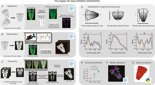
Schematic depiction of sample processing through the digital 3D-atlas making pipeline. (A) For image registration, acquired dual channel images from embryos are registered using the Fijiyama registration plugin in FIJI, the first channel (HuC:GFP signal in green) is aligned to a previously selected HuC signal which serves as reference orientation. The resulting transform file is then used to align the signal of interest (e.g. gad1b:DsRed displayed in magenta). (B) For image segmentation, Tg[HuC:GFP] embryos are used for supervised training of the Trainable Weka 3D-Segmentation algorithm. Images are provided to users, and each user inputs brush strokes on areas with signal and areas considered as background across the stack, in order to obtain a classifier (e.g. a set of filters and thresholds to be used by the algorithm to isolate the signal). Users’ generated classifiers are compared by quantification of a dozen of HuC-signals from various embryos. User classifiers resulting in more than 10% variability among users (ANOVA test) are considered outliers (e.g. u4, user 4) and are not used for sample segmentation. For each embryo, as many 3D-binary masks as user-generated classifiers are created. (C) For processing, 3D-binary masks of a single embryo are averaged to obtain a users’ average segmentation; this allows to assess the interuser segmentation variability and limits the human bias introduced by the supervised training. Signal similarity threshold between users can then be selected (here, consensus among all users was isolated). Users’ average embryo 3D-models of a given condition (n=5) are then averaged together to obtain the embryo’s averaged label. To select sample consensus threshold, we compare embryos’ averaged labels at different thresholds with their negative imprint onto the neuronal differentiation domain. Signal consensus among at least three embryos seems to recapitulate best the original signal, with marginal overlap between the signal and its imprint. Sample consensus threshold is then applied to the embryos’ averaged label to generate the final 3D-model, ready for the integration into the atlas. Several functions can be performed with DAMAKER such as (D) quantification of the signal ratio along body axes by virtually reslicing embryos’ averaged models along the desired axis, (E) quantification of users’ averaged label volumes and display them as a ratio of signal over the neuronal differentiation domain, (F) intersection of the 3D-model integrated in the atlas to assess overlapping or segregation of signals, and (G) analysis of the tissue shape.
|
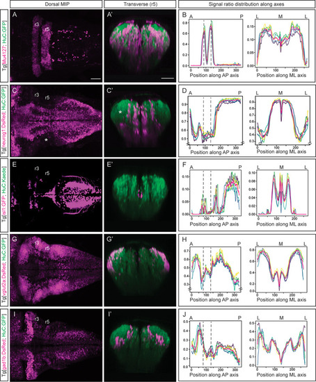
(A, C, E, G, I) Dorsal maximal intensity projections (MIP) with anterior to the left, and (A’, C’, E’, G’, I’) transverse views through r5 of registered embryos, in the Tg[HuC:GFP] background (72hpf). (A, C, E, G, I) display only the magenta signals such as r3 and r5 (Mu4127), neurog1, isl1, vglut2a and gad1b, whereas (A’, C’, E’, G’, I’) display these signals and the HuC (green). Scale bar, 50μm. (B, D, F, H, J) Signal ratio distribution along the anteroposterior (AP) and mediolateral (ML) axes of different individual embryos (n=5; colored lines), with the average value displayed as magenta line. Position along the AP and ML body axes is indicated on the top of the graph. Black dashed lines parallel to the Y-axis correspond to r3 and r5 positions assessed by Mu4127 signal. Note in (D, H) the offset in the Y-axis for easier readability of the signal variations. Scale bar, 50μm.
|
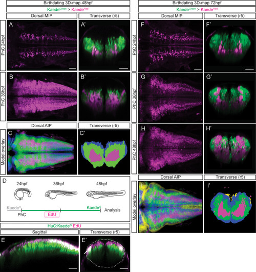
(A–B) Dorsal maximal intensity projections (MIP) showing only the HuC:KaedeRed, and (A’–B’) transverse views through r5 displaying both HuC:KaedeGreen and HuC:KaedeRed at 48hpf. HuC:KaedeGreen was photoconverted at the indicated times (PhC). Note that HuC:KaedeRed is displayed in neurons born before the time of photoconversion, and HuC:KaedeGreen in neurons born after. (C–C’) Neuronal birthdate 3D-map at 48hpf resulting from the intersection of photoconversion 3D-models. Neurons produced before 24hpf are depicted in magenta, those produced between 24hpf and 36hpf are in green, and the blue regions display neurons produced between 36hpf and 48hpf (n=5 embryos each). (D) Scheme depicting the photoconversion experiment followed by EdU-treatment. HuC:KaedeGreen was photoconverted at 24hpf, embryos were let to develop, pulsed with EdU for 6hr at 30hpf, and imaged at 48hpf. (E–E’) Tg[HuC:KaedeGreen] embryo displaying EdU (magenta) and HuC (green) in sagittal and transverse views, respectively. Note that EdU-cells are within the most dorsal part of the hindbrain, specifically in the progenitor domain and in the dorsal HuC domain (E’, see white arrow). The contour of the neural tube in (E’) is indicated with a white dashed line. (F–H) Dorsal maximal intensity projections (MIP) showing only the HuC:KaedeRed, and (F’–H’) transverse views through r5 displaying both HuC:KaedeGreen and HuC:KaedeRed at 72hpf. HuC:KaedeGreen was photoconverted at the indicated times (PhC). (I–I’) Neuronal birthdate 3D-map at 72hpf resulting from the intersection of photoconversion 3D-models. Neurons produced before 24hpf are depicted in magenta, those between 24 and 36hpf in green, the ones between 36 and 48hpf in blue, and neurons produced between the last photoconversion (48hpf) and the time of acquisition (72hpf) in yellow (n=5 embryos each). Dorsal and sagittal views display anterior to the left. Scale bar, 50μm.
|
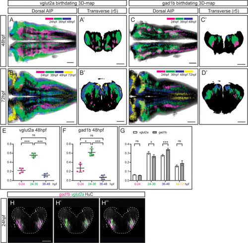
(A–D) Dorsal average intensity projections (AIP) with anterior to the left, and (A–D’) transverse views through r5, of the glutamatergic (A–B) and GABAergic (C–D) 3D-models intersected with the birthdating 3D-map at 48hpf (A, C) and at 72hpf (B, D). vglut2a or gad1b neurons produced before 24hpf, between 24 and 36hpf, between 36 and 48hpf and between 48 and 72hpf are color-coded as indicated. The differentiated domain is depicted in black. (E–F) Dot-plots showing the relative contribution to the corresponding vglut2a/gad1b-neuronal differentiation domains at 48hpf of neurons born at the indicated time intervals. (G) Interleaved bar-plot showing the relative contribution of glutamatergic and GABAergic neurons generated at different time intervals to the vglut2a/gad1b-neuronal differentiation domains at 72hpf, respectively. (E–F) RM one-way ANOVA with Tukey’s multiple comparison test, and (G) two-way ANOVA with Šídák’s multiple comparisons test; p<0.033 (*) p<0.002 (**) p<0.001 (***). (H–H’’) Transverse views of a 24hpf Tg[HuC:GFP] embryo hybridized with vglut2a (green) and gad1b (magenta), and immunostained with HuC (gray). Images are displayed as the overlay of gad1b and HuC (H), vglut2a and HuC (H’), and the merge of the three (H’’). Note that already at 24hpf, there are vglut2a and gad1b cells within the HuC domain. The neural tube contour is depicted with a white dashed line. Scale bar, 50μm.
|
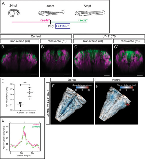
(A) Scheme with the outline of the experiment. HuC:KaedeGreen was photoconverted at 48hpf, embryos were incubated with the gamma-secretase inhibitor LY411575 during 4h, and imaged at 72hpf. As control, HuC:Kaede photoconverted non-treated embryos were used. (B–C, B’–C’) Transverse views through r3 and r5 of control (B–B’) and LY411575-treated (C–C’) embryos. Note the increase of the HuC:KaedeGreen domain upon conditionally inhibiting Notch-signaling, and the consequently remodeling of the HuC:KaedeRed domain. (D) Dot-plot displaying the neuronal differentiation volume in control and LY411575-treated embryos (n=5 embryos each). Welch’s two-tailed t-test; P<0.002 (**). Note the increase upon Notch-inhibition. (E) Quantification of the HuC:KaedeGreen volume in control and treated embryos along the ML axis. Note the accumulation of neurons in the medial differentiation domain of treated embryos. The average value is displayed as solid line and the non-linear regression as dashed line (n=5 embryos each). (F–F’) Shape comparison analysis of the neuronal differentiation domain between control and LY411575-treated embryos. Overlay of total 3D-neuronal volumes of control and treated embryos in dorsal (F) and ventral (F’) views. Color-coded legend indicates the signed distance between the two conditions. Note that the dorsal part is bluer compared with the ventral part, due to the accumulation of more neurons in this domain (n=5 embryos each). Scale bar, 50μm.
|