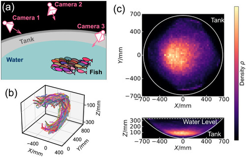
A: Schematic illustration of the experimental setup. Zebrafish were transferred into a bowl-shaped tank and three cameras were mounted above the air-water interface to record the trajectories of the fish. B: 3D trajectories obtained from the synchronised videos of different cameras. These trajectories belong to 50 young zebrafish (group Y1) in 10 seconds. C: The spatial distribution of 50 young fish (Y1) during a one-hour observation. Brighter colour indicates higher density. The top panel shows the result in XY plane, obtained from a max-projection of the full 3D distribution. The bottom panel shows a max-projection in the XZ plane. The outline of the tank and water-air interface, obtained from 3D measurement, are labelled.

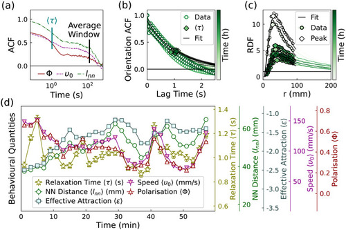
A: The auto–correlation function of the polarisation and average speed of the fish group. B: The auto–correlation function of the orientations of fish. C: Sequence of radial distribution functions with increasing time: at early times (top curves) the fish are clustered together so that the peak is large; at later times (bottom curves) the local density decreases and so does the peak height. D: The time evolution of the averaged behavioural quantities for 50 young fish. Each point corresponds to the average value in 2 minutes. The error bars illustrate the standard error values

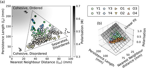
A: The states of the fish represented by the nearest neighbour distance and the persistence length. The brightness of the markers corresponds to the value of the polarisation. Each scatter–point corresponds to a time-average of 2 minutes. Different shapes indicate different fish groups from different experiments. B: A multilinear regression model fitting the relationship between the polarisation and the two length scales, indicating the polarisation increase with the increase of persistence length, and the decrease of the nearest neighbour distance. The model is rendered as a 2D plane, whose darkness indicates the value of polarisation.

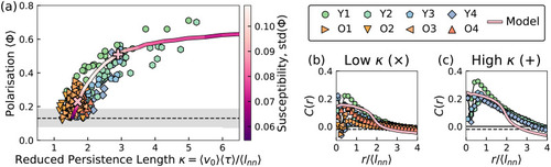
A: The average polarisation 〈Φ〉 as a function of the reduced persistence length κ, where most data points collapse, and agree with the simulation result of the inertial Vicsek model. The dashed line and grayscale zone represent the expected average value and standard deviation of 〈Φ〉 for the uniform random sampling of vectors on the unit sphere. B: The velocity correlation function of the fish and the model in the low κ states, highlighted in A with a × symbol. C: The velocity correlation function of the fish and the model in the high κ states, highlighted in A with a + symbol.