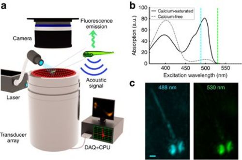
FONT set-up. (a) The imaged sample is placed in the vicinity of the geometrical center of a custom-made spherical ultrasound detection array. Light illumination of the entire object is provided via an optical fiber bundle. The generated optoacoustic signals are acquired by the array transducer, whereas the induced fluorescence is simultaneously recorded by the high-speed sCMOS camera. (b) Spectral dependence of the absorbance on calcium-bound versus calcium-free GCaMP5G (reproduced from Ref. 12). (c) Optoacoustic images of a 5-day-old HuC:GCAMP5G larva acquired at 488 and 530 nm (maximal intensity projection views through volumetric reconstructions are shown). Whereas the pigmented eyes are strongly absorbing at both wavelengths, GCaMP5G is hardly absorbing at 530 nm; thus, neural tissue is much more visible at 488 nm (scale bar=250 μm).

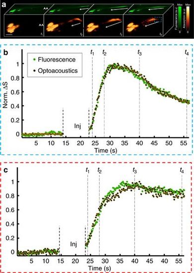
Imaging of neuronal activation in HuC:GCAMP5g zebrafish larvae. (a) Planar epifluorescence (green) and 3D optoacoustic (absorption contrast, orange) images of a 6-day-old larvae at four time points after injection of neurostimulant show a similar dynamics of the signals (scale bar=500 μm). The arrows show direction of the activation as it progresses from the posterior (site of injection marked by a double arrow in the left frame) to the anterior part of the tail. Eyes are marked with a dotted line. (b) Traces of the fluorescence and optoacoustic signals recorded at 25 frames per second show calcium dynamics in the posterior region of the spinal cord (marked by red rectangle in a). (c) Corresponding traces in the anterior region (marked by the blue rectangle). The time points shown in a are marked by vertical dotted lines. Since both the background fluorescence and optoacoustic signals were close or below the noise level, the changes in the signals (ΔS) were normalized to unity instead of being divided by the respective resting signals. The injection phase caused image artifacts and is therefore excluded from the graphs.

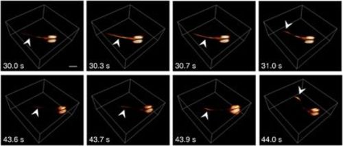
Activation in freely swimming larvae. Two separate activation events, as captured by volumetric optoacoustic tomography, are shown. Following injection of the neurostimulating agent at approximately t=0, the larva occasionally stops swimming while experiencing a surge of activation through its tail (the arrows point to the location of optoacoustic signal increase) before it starts moving promptly to a new position (notice movement of the tail in the two rightmost frames). Scale bar=500 μm.

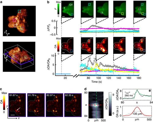
Monitoring activity in isolated scattering adult brains. (a) Typical 3D optoacoustic image acquired from a highly scattering brain of an adult fish in its resting state (two side views and one isometric view of the 3D reconstruction are shown). The telencephalon (T) and most of the optic tectum (OT) are clearly visible. Five 0.3 × 0.3 × 0.3 mm³ VOIs were chosen at different locations and depths within the brain. (b) Traces of the fluorescence (top) and optoacoustic (bottom) signal changes recorded at 25 frames per second are shown for the five regions in corresponding colors (all signal changes are normalized to the resting signal levels). Note that the optoacoustic traces are calculated over volumes, whereas the fluorescent signals are calculated over the roughly corresponding planar areas. Snapshot images (not normalized) acquired at five different time points before and after introduction of the neurostimulant are further shown (scale bar=500 μm). The volumetric optoacoustic images are shown here as maximum intensity projections along the z axis. The injection phase caused image artifacts and is therefore excluded from the graphs. (c) Time-resolved images from a single (unaveraged) slice through the 3D optoacoustic data. Approximate location of the slice is indicated by a blue frame in a. (d) Close-up spatiotemporal resolution analysis of a single line (orientation of the line is shown by an arrow in c). (e) Temporal and spatial profiles through the image in d, revealing characteristic optoacoustic signal constants of 260 ms and 135 μm, respectively. Solid green and red lines correspond to fits through the individual data points.