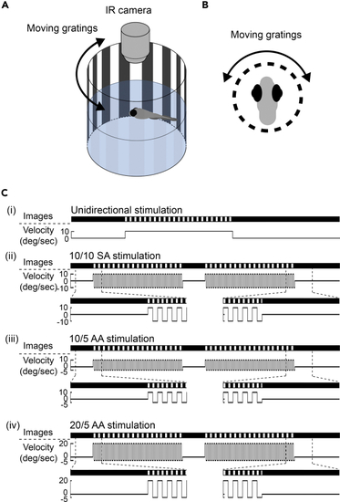
Experimental design to elicit optokinetic set-point adaptation in larval zebrafish

(A and B) Experimental setup of eye recording in larval zebrafish. Individual larval zebrafish were restrained with agarose and placed in the middle of an optokinetic cylinder. Optokinetic nystagmus (OKN) was elicited by moving gratings projected on the cylinder and recorded by an infrared (IR) camera on top of the fish.

(C) From top to bottom, schematic illustrations show optokinetic stimulations with (i) unidirectional +10 deg/sec, (ii) +/−10 deg/sec symmetric alternating (10/10 SA), (iii) +10/−5 deg/sec asymmetric alternating (10/5 AA), and (iv) +20/−5 deg/sec asymmetric alternating (20/5 AA) stimulus velocities. Under all stimulus conditions, a 5-min pre-stimulus dark period and a 10-min post-stimulus dark period were included. Stimulus duration was 10 min for (i) and twice 20 min with a 5-min inter-stimulus dark period for (ii)-(iv).

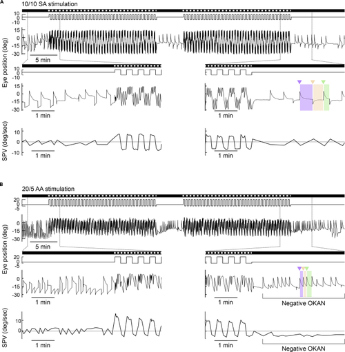
Negative OKAN can be elicited by asymmetric optokinetic stimulation

(A and B) Typical eye-position traces with corresponding slow-phase velocities (SPVs) of zebrafish larvae under 10/10 symmetric alternating (SA) (A), and 20/5 asymmetric alternating (AA) (B) stimulations. The SPV was estimated as the median velocity in the first second of each slow phase (shaded area) after discarding the quick-phase eye movement (triangle). The stimulus image pattern (darkness or gratings) and the stimulus velocity are shown on the top as horizontal bars and lines, respectively. At the bottom, the magnified traces are shown to better demonstrate the transition phases from pre-stimulatory darkness to optokinetic nystagmus (OKN) and from OKN to post-stimulatory darkness. Positive values represent movements to the left (counterclockwise), and negative values represent movements to the right (clockwise).

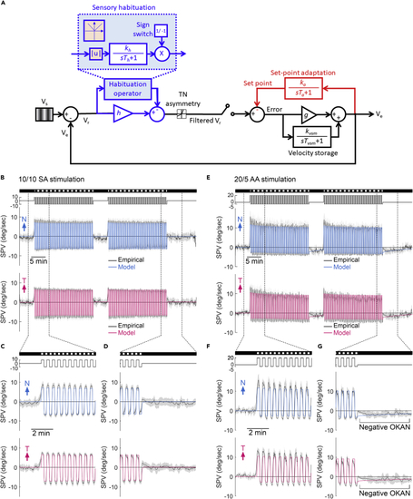
Optokinetic set-point adaptation model predicts the recorded SPV in larval zebrafish

(A) The mathematical model of set-point adaptation. Retinal slip velocity (V_r) is the difference between the stimulus velocity (V_s) and the eye velocity (V_e). During habituation, V_r is rectified and filtered with a time constant of T_h and gain of k_h (blue shaded area), and then scaled with h, to give a filtered V_r. In the sensory habituation operator, |u|, which produces the absolute value of the input (orange shaded area), together with a sign switch of output lead to a continuous habituating effect regardless of stimulus direction. The filtered V_r passes through a nonlinear gain (T-N gain) that captures the T-N asymmetry. The error between the filtered V_r and the set point is scaled by oculomotor gain (g) and added to the velocity storage mechanism (VSM) to control V_e. VSM contains a leaky integrator with a time constant of T_vsm and a gain of k_vsm that contributes to the eye velocity. V_e is then integrated with a time constant of T_a and a gain of k_a to adjust the set point.

(B–G) The model predicted population-median SPV (colored lines) superimposed on the median ± median absolute deviation (black line with gray shadow) of empirical SPVs during 10/10 symmetric alternating stimulations (SA, n = 29) (B–D) and 20/5 asymmetric alternating stimulations (AA, n = 18) (E–G). Considering the starting direction of alternating stimulation was randomized, we aligned the first stimulus direction as positive instead of left or right. Therefore, the plots show one eye started with a nasalward movement (blue trace) and another eye started with a temporalward movement (red trace). The stimulus image pattern (darkness or gratings) and the stimulus velocity are shown on the top as horizontal bars and lines, respectively.

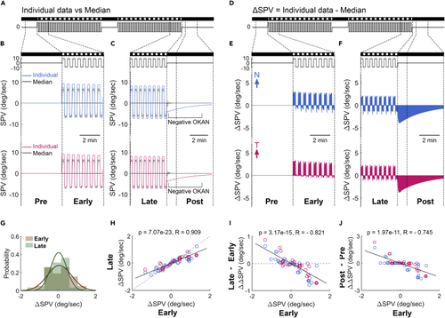
Zebrafish larvae display different levels of asymmetric OKN under the symmetric stimulus

(A) A typical eye-position trace of a single larva with an asymmetric optokinetic nystagmus (OKN) under 10/10 symmetric alternating (SA) stimulation and the following negative optokinetic afternystagmus (OKAN). The bottom plots show magnifications to demonstrate the transition phases from OKN to inter- and post-stimulatory periods, respectively.

(B and E) The stimulus image pattern and the stimulus velocity are shown as horizontal bars and lines, respectively.

(C and D) The slow-phase velocity (SPV) of (A, color line) is compared to the median ± median absolute deviation of 29 subjects (black line with gray shadow).

(F and G) The difference in SPVs between the individual larva (color line in C and D) and the population median (black line in C and D). Dashed lines extend from (E) to (F and G) illustrate the time windows for further analyses in (H–K).

(H) The ΔSPV probability distribution of 29 fish during the early and late periods. Two lines demonstrate the fit of distributions with Gaussian function.

(I) The late ΔSPV plotted over the early ΔSPV. The slope of the linear regression line (solid line) is significantly smaller than 1 (p = 1.79e-08; interactive analysis of covariance) and the slope of the dashed line (temporally shuffled data; p = 4.21e-06; interactive analysis of covariance).

(J) The changes in ΔSPV across stimulus phases (late ΔSPV – early ΔSPV, ΔΔSPV) plotted over the early ΔSPV. The slope of linear regression line (solid line) is significantly lower than the slope of the dashed line (temporally shuffled data; p = 4.21e-06; interactive analysis of covariance).

(K) The changes of the eye movements in the dark before and after OKN (post-ΔSPV – pre-ΔSPV, ΔΔSPV) plotted over the early ΔSPV. Filled circles represent the data of the animal shown in (A). Black solid lines demonstrate the linear regression fit of recorded data. Considering the starting direction of alternating stimulation was randomized, we aligned the first stimulus direction as positive instead of left or right. Therefore, the plots show one eye started with a nasalward movement (blue trace) and another eye started with a temporalward movement (red trace). p, p values; Pearson correlation. R, correlation coefficients; Pearson correlation.

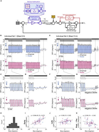
An innate bias in the optokinetic system accounts for the asymmetric OKN and the corresponding set-point adaptation under the symmetric stimulus

(A) A modified mathematical model to explain the asymmetric optokinetic nystagmus (OKN) gain under symmetric stimulation and the following optokinetic afternystagmus (OKAN). The design is based on the proposed model shown in Figure 3A; however, a constant innate bias (yellow box) is introduced to the optokinetic system.

(B–G) The model predicted slow-phase velocity (SPV, colored lines) superimposed on the empirical SPVs of individual subjects (black lines) with symmetric (B–D) and asymmetric (E–G) eye movements.

(E) is the same data shown in Figure 4A. Considering the starting direction of alternating stimulation was randomized, we aligned the first stimulus direction as positive instead of left or right. Therefore, the plots show one eye started with a nasalward movement (blue trace) and another eye started with a temporalward movement (red trace). The stimulus image pattern (darkness or gratings) and the stimulus velocity are shown on the top as horizontal bars and lines, respectively.

(H) The fish counts of the estimated bias (total fish number = 29).

(I–K) The early ΔSPV (I), late ΔSPV (J), and the changes of the eye movements in darkness before and after OKN (post-ΔSPV – pre-ΔSPV, ΔΔSPV) (K) plotted over the estimated bias. V_s, stimulus velocity. V_e, the eye velocity. V_r, the retinal slip velocity. V_e, eye velocity. T_h, habituation time constant. k_h, habituation gain. |u|, absolute operator. g, oculomotor gain. T_vsm, velocity storage time constant. k_vsm, velocity storage gain. T_a, set-point adaptation time constant. k_a, set-point adaptation gain. p, p-values; Pearson correlation. R, correlation coefficients; Pearson correlation.

The model is generalizable across individuals

(A and D) The stimulus image pattern and the stimulus velocity are shown as horizontal bars and lines, respectively.

(B and C) The simulated slow-phase velocity (SPV) of Figure 4A (color line) is compared to the median ± median absolute deviation of simulations from all 29 subjects (black line with gray shadow).

(E and F) The difference of SPVs between the individual simulation (color line in B and C) and the population median (black line in B and C). Dashed lines extend from (D) to (E and F) illustrate the time windows for further analyses in (G–J).

(G) The ΔSPV probability distribution of 29 fish during the early and late periods. Two lines demonstrate the fit of distributions with Gaussian function.

(H) The late ΔSPV plotted over the early ΔSPV. The slope of linear regression line (solid line) is significantly smaller than 1 (p = 5.58e-19; interactive analysis of covariance) and the slope of the dashed line (temporally shuffled data; p = 1.94e-18; interactive analysis of covariance).

(I) The changes in ΔSPV across stimulus phases (late ΔSPV – early ΔSPV, ΔΔSPV) plotted over the early ΔSPV. The slope of linear regression line (solid line) is significantly lower than the dashed line (temporally shuffled data; p = 1.94e-18; interactive analysis of covariance).

(J) The changes of the eye movements in the dark before and after optokinetic nystagmus (post-ΔSPV – pre-ΔSPV, ΔΔSPV) plotted over the early ΔSPV. Filled circles represent the data of the animal shown in (A–F).

(H and I) Black solid lines demonstrate the linear regression fit of simulated data. Considering the starting direction of alternating stimulation was randomized, we aligned the first stimulus direction as positive instead of left or right. Therefore, the plots show one eye started with a nasalward movement (blue trace) and another eye started with a temporalward movement (red trace). p, p values; Pearson correlation. R, correlation coefficients; Pearson correlation.