
- Title
-
Ancestral circuits for vertebrate color vision emerge at the first retinal synapse
- Authors
- Yoshimatsu, T., Bartel, P., Schröder, C., Janiak, F.K., St-Pierre, F., Berens, P., Baden, T.
- Source
- Full text @ Sci Adv

In vivo spectral tuning of larval zebrafish cones and HC block. (A) Schematic of larva zebrafish retina, with position of cone pedicles highlighted [adapted from (82)]. (B and C) Example scans of the four spectral cones (B) (Methods) with single pedicle response examples for each (C) to 3-s flashes of light from each of the 14 LEDs [see fig. S1 (A to C)]. The means superimposed on individual repeats are shown. (D) Example spectral responses summarized from (C). Note that in this representation, both the x and y axes are flipped relative to the raw responses. (E and F) Population responses of each cone type recorded in different parts of the eye (D, dorsal; N, nasal; AZ, acute zone; V, ventral; see schematic inset above for anatomical reference; vertical scale bars indicate n = 100 cones; see also fig. S1G) (E) and population mean ± 95% confidence intervals with log-transformed respective opsin template superimposed (F) (Methods). Heatmaps (E) are time-inverted to facilitate comparison to summary plots (F); grayscale bars are in z scores. Darker shades indicate a drop in calcium relative to baseline, indicative of a cone’s “intrinsic” light response, while lighter shades indicate a rise in calcium, indicative of sign-inverted inputs from the outer retinal network (see Fig. 2). |

Opsin-like cone responses in the absence of HCs. (A and B) Population responses of each cone type during pharmacological blockage of HCs (A) (Methods) and population mean ± 95% confidence intervals with log-transformed respective opsin template superimposed (B) (Methods). (C) Pharmacogenetic UV cone ablation in the background of red cone GCaMP labeling before (top) and 24 hours after 2-hour treatment of metronidazole (10 mM) application (bottom) (Methods). (D and E) Red cone tunings after UV cone ablation (n = 77) (D) and after additional pharmacological HC blockage (n = 103) (E). Heatmaps (left) and means ± SD (solid lines and shadings) and analogous data in the presence of UV cones (dotted, from Figs. 1F and and2B)2B) are shown. Note that the 361-nm LED was omitted in this experiment. (F) As (D), but here, recording from blue cones (n = 30). (G and H) Red (n = 17) (G) and UV cone tunings (n = 43) (H) at about ninefold reduced overall stimulus-light intensities (solid lines and shadings; Methods), compared to tunings at “standard” light intensities (from Fig. 1F). Gray bars on the x axis in (D) to (H) indicate significant differences based on the 99% confidence intervals of the fitted generalized additive models (GAMs) (Methods). Note that heatmaps (A and D to H) are time-inverted to facilitate comparison to summary plots (B and D to H). Grayscale bars are in z scores. |
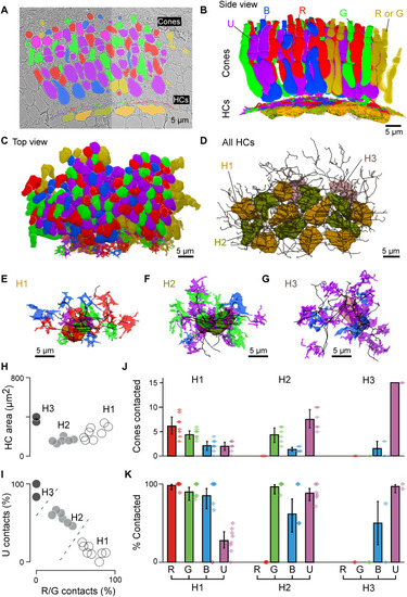
Connectomic reconstruction of outer retinal circuitry. (A) Example vertical EM section through the outer retina, with cones and HCs painted. Cones are color coded by their spectral identity, with “yellow cones” indicating red or green cones at the section edge that could not be unequivocally attributed (Methods); HCs: H1, yellow/brown; H2, dark green; and H3, light pink. (B to D) Full volumetric reconstruction of all cones and skeletonized HCs in this patch of retina, shown from the side (B), top (C), and HCs only (D). (E to G) Example individual HCs classified as H1 (E), H2 (F), and H3 (G) with connecting cone pedicles. (H to K) Quantification of HC dendritic area (H) (cf. fig. S3G) and cone contacts (J and K) shown as absolute numbers with bootstrapped 95% confidence intervals (J) and percentage of cones in dendritic territory with binomial confidence intervals (I and K). |

Spectral tuning of cones by HCs. (A to E) Linear model of spectral tuning in an outer retinal network composed of four cone types and three HC types, with maximum connectivity matrix defined as in Fig. 3K (Methods). Cone tunings are initiated on the basis of in vivo data during HC block (Fig. 2B). Different HC combinations include (A) (from left) the following: no HCs, all HCs, and H1 only. In each case, the model computes resultant cone tunings (solid lines) superimposed on in vivo data in the absence of HC block (shadings, from Fig. 1F) (B) and reconstruction quality (C) as loss relative to the peak performance for the full H1 to H3 model (loss = 0) and in the absence of HCs (loss = 1) and normalized weights such that cones contributing to a given HC, and HCs contributing to the full model, each add up to 1 (D). In addition, resultant HC tunings are shown for the full H1 to H3 model (E). (F to J) In vivo voltage imaging of HC somata’s spectral tuning (Methods). (F and G) Example scan (F) [average image (top) and local response correlation (83) and regions of interest (ROIs; bottom)] and responses (G) (mean superimposed on individual repeats shown for the three HC somata in this scan, of which ROIs 1 and 2 responded broadly across all tested wavelength, while ROI 3 exhibited a clear short-wavelength preference). (H to J) Results of clustering of mean responses from n = 86 ROIs (H) (n = 15 fish) with cluster means (I) and extracted tuning functions (J) (means ± SD). (K and L) Mean tunings of in vivo HC clusters [(K), from (J)] and superposition of each modeled [solid lines, from (E)] and measured [shading, from (K)] HCs. Note that raw (G) and averaged (I) HC responses and the summary heatmap (H) are time inverted to facilitate comparison with summary plots (J to L). The grayscale bar in (H) is in z scores. |

In vivo cone tunings efficiently represent statistics of natural light. (A to C) Hyperspectral data acquisition from zebrafish natural visual world. A 60° window around the visual horizon of an example scene recorded in the zebrafish natural habitat (A) was sampled at 1000 equispaced points with a custom-built spectrometer-based scanner (13) (B) to yield 1000 individual spectral readings from that scene. (C) Summary of the pooled and z-normalized data from n = 30 scenes (30,000 spectra) with mean ± SD [data from (14)]. Photo credit (A): Tom Baden, University of Sussex. (D to L) Reconstructions and analysis of the example scene as seen through different spectral filters: (D to F) log-opsin spectra, (G to I) cone in vivo tunings, and (J to L) based on the first three PCs that emerge from the hyperspectral data shown in (C). From left to right: (D, G, and J) example scene [from (A)] reconstructed on the basis of opsin/in vivo/PC tunings as indicated, (E, H, and K) correlation matrices between these respective reconstructions, and (F, I, and L) the actual tunings/PCs. A fifth element GB (for “green/blue”) is computed for in vivo tunings as contrast between green and blue cone tunings (cf. fig. S5). (M) Percent variance explained by the first five PCs (l). (N) Superposition of cone in vivo tunings (colored lines), PCs, and a linear R/G/B/U log-opsin fit to the respective PC (yellow; Methods). The latter fit can be seen as the biologically plausible optimum match to a given PC that can be achieved in a linear regime. |

Encoding of natural achromatic and chromatic contrast. (A) Computed responses of in vivo cones, the GB axis, and each respective log-opsin PC fit [all from Fig. 5 (I and N)] to each of the n = 30,000 individual natural spectra, plotted against each spectrum’s loadings onto PC1 (top row), PC2 (middle row), and PC3 (bottom row), as indicated. Responses were plotted on the y axis, and PC loadings were plotted on the x axis. In general, a column that shows a near-perfect correlation in one row, but no correlation in both other rows (e.g., column 1), can be seen as a tuning function that efficiently captures the respective PC (e.g., column 1 shows that red cones efficiently represent PC1 but not PC2 or PC3). (B) Corresponding summary statistics from (A), based on scene-wise Spearman correlations. (C) Spectral tuning functions of Drosophila R7/8 photoreceptors as measured in vivo at their synaptic output [data from (12)]. (D) Comparison of Drosophila tuning functions with the first three PCs that emerge from terrestrial natural scenes [data from (13)]. Here, PC3 is matched with a yyp8 axis as indicated [cf. fig. S6 (D to F)]. (E) Summary stats of Drosophila photoreceptor responses to each of the n = 4000 individual terrestrial natural spectra plotted against their respective PC loadings. |