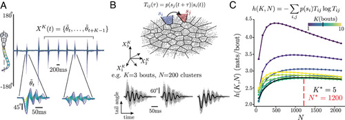
Building a maximally predictive state space for larval zebrafish. (A) Typical example of larval zebrafish locomotion bouts, measured as the cumulative angle made by points on the tail with respect to the midline. An example turn (Left) and forward (Right) bout are shown below. We construct bout sequences (gray bar), increasing the sequence length to maximize predictability. (B) Illustration of the estimation of transition matrices as a function of the number of bouts in a sequence and the number of partitions . We cluster the bout sequence space into discrete microstates and estimate transition probabilities (SI Appendix). Below, we illustrate an example microstate constructed with , : We plot the cumulative tail angle in the bout sequences belonging to the microstate (gray, average in black). (C) To probe the short-time predictability of the dynamics across sensory contexts, we estimate the entropy rate of the transition matrix constructed with for varying and (we sample 7,500 bouts from each sensory context from ref. 11; see SI Appendix). Increasing offers resolution over the bout sequences, while increasing offers predictability. We choose to minimize the entropy rate, and choose to maximize the resolution before finite-size effects result in the underestimation of the entropy rate (33).

Zebrafish navigation is led by long-lived modes with a hierarchy of timescales prioritizing change of orientation, speed, and egocentric direction bias. (A) Implied timescales of the -th mode of the reversibilized , estimated as , where are the eigenvalues of with , SI Appendix, Fig. S2A. We find three long-lived modes that are well separated from the bulk spectrum, while faster modes are closer to each other. Error bars are bootstrapped 95% CI obtained by sampling 7,500 bouts from each 14 sensory context (11) over 100 seeds (SI Appendix). (A, Inset) We show the averaged transition matrix . (B) Microstates projected along and color coded by the mean absolute change in heading for the bouts belonging to each of the microstates. Increasing is associated with higher amplitude reorientations. (C) Same as (B), but color coded by the mean speed in each microstate . We find that higher is generally associated with higher speeds. (D) Probability density of the mean change in heading for each of the microstates along the third mode . Low values of correspond to leftward bouts, while high values of correspond to rightward bouts. (E) Cumulative distribution function (CDF) of the absolute mean change in heading direction for all bouts belonging to the cruising (red) and wandering (blue) strategies, identified by partitioning along (SI Appendix). (E, Inset) Reorganized , where each microstate in cruising or wandering is placed together, revealing a block diagonal structure. (F) Mean sequence length (MSL) of fish in wandering and cruising strategies. We infer a coarse-grained transition matrix among cruising and wandering , and simulate sequences by sampling the next state according to the transition matrix (SI Appendix). We find that the coarse-grained Markov models inferred for each fish accurately predict the mean sequence lengths in cruising and wandering. Note also the wide variability in mean sequence lengths among fish, from a few bouts to a few hundreds of bouts.

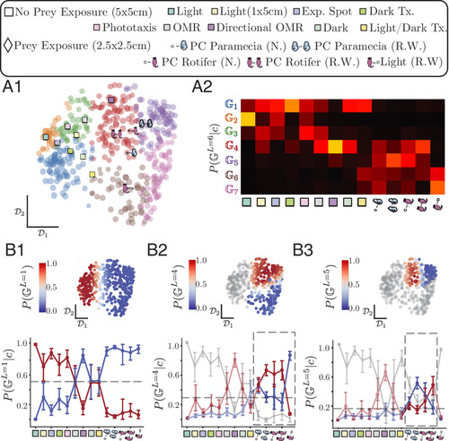
Preferences for distinct motor strategies are deployed across sensory contexts. (A) Left, probability density of visiting microstates along . Right, example trajectory color coded by (Top) and median dwell time in each strategy (Bottom) (error bars represent 95% CI bootstrapped across fish, with individual fish scattered in the background). (A1) In large square arena in the light, fish mostly fast cruise ( , , 10 fish). (A2) In a smaller arena, fish in the light use wandering at the short ends when forced to reorient ( , arena, 12 fish), resulting in a reduction of time spent cruising compared to (A1). (A3) In the dark, fish show a shift toward fast wandering ( , 37 fish, data combined from the “Dark” condition and the first 30 min of the “Dark Transitions” condition; see SI Appendix, Table S1). (A4) In a prey capture assay with 50 paramecia per arena, fish mostly engage in slow cruising and wandering when the eyes are converged, and introduce faster wandering when the eyes diverge ( , arena, 65 fish). Each bout is given an eye convergence index based on the angle between the eyes (SI Appendix). Note the near absence of fast cruising when compared to (A1). (B) Probability of hunting (B1) or detecting (B2) resources in each of the motor strategies, SI Appendix, Fig. S3D1. Using data from all fish, we infer transition matrices using only the microstates belonging to each motor strategy and simulate trajectories (SI Appendix, Fig. S5). (B1) We assess the fish’s ability to hunt prey that is uniformly distributed within cone of aperture ahead of its head (eyes converged) (40) and radius. We simulate fish trajectories for the average duration of hunting sequences ( ), SI Appendix, Fig. S5A, and count successful hunts when the head trajectory is within from the prey ( 5% of the body length); see SI Appendix. In this case, slow cruising is the most successful strategy. (B2) We assess the fish’s ability to detect resources uniformly scattered within a distance from the initial position (41) We now simulate 1,000 bout-long trajectories, and assume that the fish can detect resources within a distance around its head position (SI Appendix). In this case, the wandering states are most effective up to mesoscale search ( ) while fast cruising is effective at large scale dispersal. The black line represents the behavior of an average fish. Errorbars and shaded areas correspond to bootstrapped 95% CI obtained from 10,000 simulations from random initial conditions.

Sensory contexts cannot fully explain behavioral variability across fish. We encode the behavior of each fish in transition matrices built with an increasing number of coarse-grained states , and use regularized logistic regression to classify each fish to their respective sensory contexts. (A) Accuracy of the classification task (fraction of correct classifications) for the Train (black) and Test (yellow) sets plotted as a function of the number of coarse-grained states (SI Appendix): the Train accuracy grows continuously as a function of and rapidly reaches while the test accuracy reaches only , far from perfect. Minimal improvements are seen above above which the classifier overfits. states correspond to Left–Right variations of slow-fast cruising–wandering motor strategies (Right, example trajectories). (B) Confusion matrix of the classifier for in which each row reflects the proportion of individuals assigned from each sensory context to all conditions. A strong diagonal component indicates that a large portion of fish are correctly assigned, while off-diagonal components point to fish misclassified into a different sensory context. Sensory contexts with visual stimuli are labeled with squares while prey exposure conditions are labeled with a diamond.

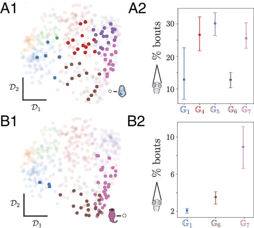
Phenotypic groups emerge by clustering individual fish based on their behavioral dynamics. (A) Pairwise distance matrix between the transition matrices of individual fish at . We find structure across multiple scales, with prey exposure being an important source of variability. (B) We use a constant shift embedding (CSE) to map distances onto an Euclidean space that preserves the pairwise distances among individual fish (gray dots). We plot the first two dimensions of the transition matrix space with example matrices displayed for two individuals (red dots). We test whether two fish behave significantly differently over the experimental timescale by re-estimating transition matrices from finite simulations of each fish’s and calculating the distance between the re-estimated and original transition matrices (blue area around example fish). Averaging these distances sets an effective scale (blue area around example fish) within which neighboring fish are indistinguishable from each other (SI Appendix). (C) Left, illustration of our clustering approach as a tree diagram, with the distance matrix organized according to the cluster assignment. We structure the phenotypic space through a top–down subdivision of a multiplicative diffusion process [hierarchical multiplicative diffusive (HMD) clustering] where distances are rescaled by . At each iteration , the group of fish that is most separable is subdivided so that the ordering of subdivisions is indicative of the relative scale separation among fish from different groups. We stop the clustering at the point beyond which the effective distances between fish within clusters stop decreasing ( , 7 clusters, vertical dashed line; see SI Appendix, Fig. S6B). The widths of the branches of the tree are proportional to the number of fish in each cluster. (C) Right, individual fish are color-coded by their most likely phenotypic group , where . Dot size indicates the posterior probability . (D) Clustering reveals different phenotypic groups : Groups exhibit a bias toward fast cruising (with also exhibiting fast wandering and also exhibiting slow cruising and wandering) while groups share a bias toward slow cruising and wandering (with exhibiting also faster cruising) and groups use mostly fast wandering, with some slow cruising and wandering also for . (E) Probability of either hunting (E1) or detecting (E2) resources for the phenotypic groups, as in Fig. 3B (SI Appendix, Fig. S5). (E1) Probability of hunting prey within 3 bouts (SI Appendix, Fig. S5A), at a distance of (41) and within a cone of ahead of the fish (40): group , which biased toward slow cruising and wandering strategies, is the most effective at gathering prey. (E2) Probability of detecting uniformly distributed resources with a radius : groups are effective for short to meso-length scale search, while are most effective at large scale dispersal. Group is approximately equally efficient across a broad range of length scales (black line, average of all groups).

Phenotypic group structure reveals prey exposure as a major determinant of variation. (A1) Transition matrix space of all individuals color-coded by phenotypic groups together with the average position for each condition using symbols detailed above. (A2) Probability of a fish to belong to group in a given experimental condition , : While no sensory context maps onto a phenotypic group, most fish of a given context have preferences for specific groups: fish never exposed to prey often belong to , while fish exposed to prey often belong to groups . (B1–B3) Probability of belonging to group for fish in a condition at different iterations in the hierarchical subdivision (gray line, probability of belonging to neither of the groups): (B1) the first splits fish exposed to prey (during or prior the assay, Right in blue) from fish never exposed to prey (Left in red) (note that the OMR, Dark, and Light/Dark transitions assays are equally distributed across these two groups). (B2) The fourth subdivision distinguishes fish previously exposed to prey but swimming in the light without prey from the fish that had prey in the arena. (B3) At , we find differences stemming from the prey type and prior exposure. In the dashed box, we see that naive fish hunting for the first time split equally, whereas fish raised with either paramecia or rotifers generally belong to distinct groups.

Phenotypic group structure reveals the role of hidden internal states in structuring the behavioral variability among fish exposed to the same sensory context. (A1) Transition matrix space color-coded according to the 7 phenotypic groups, with naive fish hunting for paramecia highlighted. (A2) Fraction of bouts with high eye convergence for naive fish hunting paramecia according to the phenotypic group reveals that fish in and spent less time with eyes converged, indicating lower rate of hunting than fish in other groups. (B1) Transition matrix space color-coded according to the seven phenotypic groups, with fish exploring in the light that were previously raised with rotifers highlighted. (B2) Fraction of bouts with eye convergence across fish in the light raised in different conditions across phenotypic groups uncovers that fish in and show very little eye convergence rates, while fish in exhibit higher eye convergence, indicating that they attempt hunting more frequently. These differences indicate that phenotypic groups reflect hidden internal states impacting behavior. We estimate the eye convergence rates per fish, and show the phenotypic groups that have more than one fish with bootstrapped 95% CI obtained across fish.