Schematic illustrations of SAMPL hardware design

(A) Overview of the apparatus without aluminum rails, side panels, and the top panel. Equipment modules mounted on the breadboard are, from left to right, IR camera and lens, chamber holders, and IR illumination module.

(B) Exploded-view drawing of the IR illumination module.

(C) Exploded-view drawing of the camera and lens module.

(D) Exploded-view drawing of a chamber holder.

(E) Design of fish chambers. From left to right: 3D illustration of a standard chamber (top) and a narrow chamber (bottom), front view of the U-shaped acrylic middle piece for the chambers, and side view of the chamber. Pink squares illustrate the recording field of view. i = 20 mm; s = 1.5 mm.

(F) Dimensions of the apparatus frame and breadboard.

(G) Design and dimensions of the apparatus lid.

(H) Schematic illustration of a set of three SAMPL apparatus and a small-form-factor computer case on a 24″ × 36″ shelf.

See also Figure S1, Table S1, and Video S1.

High-definition recording and measurement of animal locomotion using SAMPL

(A) Example of a recorded frame with a Drosophila melanogaster (white box) in the SAMPL apparatus. Dashed line indicates heading of the fly relative to vertical up (north). Imaging was performed at 166 Hz with 1,200 × 1,216 pixels. Same as follows.

(B) Example of an epoch of a walking fly. Walking speed and heading are plotted as a function of time. Gray and cyan lines mark resting and grooming periods, respectively (Video S2).

(C) Example of a recorded frame with a Caenorhabditis elegans (white box) in the SAMPL apparatus. Dashed line indicates approximated angle of the worm relative to vertical.

(D) Example of an epoch of a swimming worm. z position and approximated angle are plotted as a function of time. Cyan vertical lines label the time when the plane of movement is perpendicular to the imaging plane (Video S2).

(E) Example of a recorded frame with a 7 dpf Danio rerio larva (white box) in the SAMPL apparatus. Pitch angle is determined as the angle of the trunk of the fish (dashed line) relative to horizontal. Positive pitch indicates nose-up posture, whereas negative pitch represents nose-down posture.

(F) Example of an epoch containing multiple swim bouts (arrows). Swim speed and pitch angles are plotted as a function of time. Dashed line marks the 5 mm/s threshold for bout detection. Cyan vertical lines label time of the peak speed for each bout.

See also Table S2 and Videos S2 and S3.

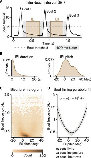
Modeling timing of swim bouts reveals larval sensitivity to pitch changes

(A) An inter-bout interval (IBI; brown area) is defined as the duration when swim speed is below the 5 mm/s homeostasis threshold (dashed line) between two consecutive bouts with a 100 ms buffer window (gray area) deducted from each end.

(B) Distribution of IBI duration (left) and mean pitch angle during IBI (right).

(C) Bivariate histogram of bout frequency and IBI pitch. Bout frequency is the reciprocal of IBI duration.

(D) Bout frequency plotted as a function of IBI pitch and modeled with a parabola (black line, R ² = 0.14, mean ± SD). Brown dots indicate binned average of IBI pitch and bout frequencies calculated by sorting IBI pitch into 3°-wide bins.

For all panels, n = 109,593 IBIs from 537 fish over 27 repeats.

See also Table S3.

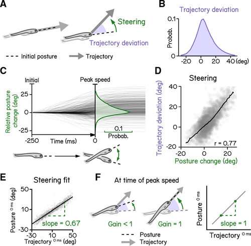
Larval vertical navigation is led by steering toward trajectory

(A) Schematic illustration of two climbing mechanics: (1) a larva may generate a thrust (arrow) toward the pointing direction (dashed line) at the initial of a bout (left), and (2) a larva can steer (green arrow) toward an eccentric angle before the thrust (right). The offset between trust angle and the direction the larva point toward at bout initial is termed trajectory deviation (purple).

(B) Distribution of trajectory deviation.

(C) Changes of pitch angles relative to initial pitch plotted as a function of time(dark lines) overlaid with distribution of pitch change at time of peak speed (green).

(D) Trajectory deviation (purple) plotted as a function of posture changes from bout initial to time of the peak speed (green). Black line indicates binned average values. Positive correlation between trajectory deviation and posture change demonstrates that larvae steer toward the trajectory of the bout.

(E) To measure the gain of steering compared with trajectory deviation, pitch angles at time of the peak speed are plotted as a function of trajectory. Steering gain is determined as the slope of the fitted line (Pearson’s r = 0.96).

(F) Schematic illustrations demonstrating how steering gain associates steering (green arrows) with trajectory deviation (purple).

For all panels, n = 121,979 bouts from 537 fish over 27 repeats.

See also Table S3.

Steering requires coordination of fin and body

(A) Swim speed (top) and angular velocity (bottom) plotted as a function of time. Angular velocity peaks (asterisk and dotted area, mean ± SD) during steering phase (green) before time of the peak speed. Angular velocity is adjusted by flipping signs of bouts with nose-down rotations during steering (mean ± SD across experimental repeats). Shaded region in the top panel indicates mean ± SD across all quantified swim bouts.

(B) Histogram of time of peak angular velocity, binned by frame, across experimental repeats with mean ± SD plotted below.

(C) Illustration of components that contribute to trajectory deviation. Larvae rotate their bodies starting from bout initial (blue) and reach peak angular velocity (asterisk) before peak speed. Any rotation generated during decrease of angular velocity is considered residual (gray). At time of peak speed, there is an offset between the pitch angle (dashed line) and bout trajectory (arrow), which is termed the attack angle (orange). Body rotations, residual, and attack angle add up to trajectory deviation.

(D) Distribution of attack angles in control fish(left) and fish after fin amputation (right). Dashed lines indicate 0 attack angle.

(E) Attack angles plotted as a function of body rotations (left, blue) or residual rotations (right). Rotations and residuals are sorted into 0.5°-wide bins for calculation of binned average attack angles. Swim bouts with negative attack angles while having steering rotations greater the 50th percentile (hollow squares) were excluded for binned-average calculation.

(F) Attack angles plotted as a function of body rotations (blue line) and fitted with a logistic model (black line, R² = 0.31, mean ± SD). Fin-body ratio is determined by the slope of the maximal slope of the fitted sigmoid (magenta). Rotations are sorted into 0.8°-wide bins for calculation of binned average rotations and attack angles (blue line). Swim bouts with negative attack angles while having steering rotations greater the 50th percentile were excluded for sigmoid modeling.

(G) Schematic illustration of how fin-body ratio reflect climbing mechanics.

For all panels, n = 121,979 bouts from 537 fish over 27 repeats.

See also Table S3.

Righting rotation restores posture after peak speed

(A) Pitch angles plotted as a function of time (dark lines) overlaid with distribution of pitch angles before (left) and after bouts (right). Red area indicates duration after peak speed when pitch distribution narrowed.

(B) Illustration of righting behavior. Larvae rotate (red arrows) toward more neutral posture after peak speed.

(C) Distribution of rotation during righting (red in A).

(D) Righting rotation plotted as a function of initial pitch angles.

(E) Righting gain is determined by the absolute value of the slope (red dotted line) of best fitted line (black line). The x intersect of the fitted line determines the set point (blue cross) indicating the posture at which no righting rotation results.

(F) Schematic illustration of righting rotation (red arrows), righting gain, and setpoint (blue dashed line).

For all panels, n = 121,979 bouts from 537 fish over 27 repeats.

See also Table S3.

Statistics of regression analysis for swim kinematics

(A) Confidence interval (CI) width of kinematic parameters plotted as a function of sample size at 0.95 significance level (mean ± SD as ribbon). Errors were estimated by resampling with replacement from the complete dataset.

(B) Effect size plotted as a function of sample size at various percentage differences. Mean ± SD.

Refer to STAR Methods for details of computation.