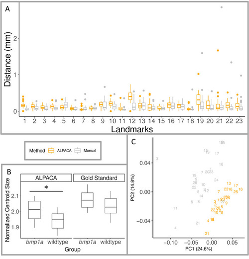
Pipeline validation using 23 traditional landmarks. Boxplots are shown for (A) Euclidean distance between Gold Standard landmark locations and ALPACA transferred points (orange), and distance between the two manual landmark placements (grey), where color indicates method used for all panels, and (B) normalized centroid size of gold standard and ALPACA transferred pseudo-landmarks. Midline of boxplots show median value, with hinges corresponding to first and third quartiles, and whiskers extending to largest and smallest value no further than 1.5 times the interquartile range. Also shown (C) are the first two principal components of shape space from the combined GPA analysis of gold standard and ALPACA transferred 23 landmarks. The percent of variance for each PC is show in parenthesis of each axis. Individual fish are depicted as different numbers, fish 1–12 are crispant fish, fish 13–26 are wild-type fish, and fish 27 is the atlas.

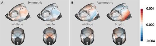
Heat map of (A) symmetric and (B) asymmetric components of shape variation. Lateral and anterior views are shown for each group (wild type and bmp1a) within both components of shape variation. Colors show variation in shape from the symmetric atlas, with deeper colors representing greater variation from the atlas.

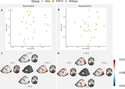
First two principal components of symmetry analysis. PC plots show separation of groups (represented by color) along the first and second PCs (A,B). Heat maps of the same PCs represent where shape variation occurs across each axis (C,D). Columns represent symmetric (A,C) and asymmetric (B,D) components of shape variation. The central image in C and D represents mean shape of each component. Color in C and D represents the Procrustes distance between the average shape and the shape occupying the ends of each PC axis. Deeper colors represent larger differences, and the specific colors refer to differences in direction relative to the average image.

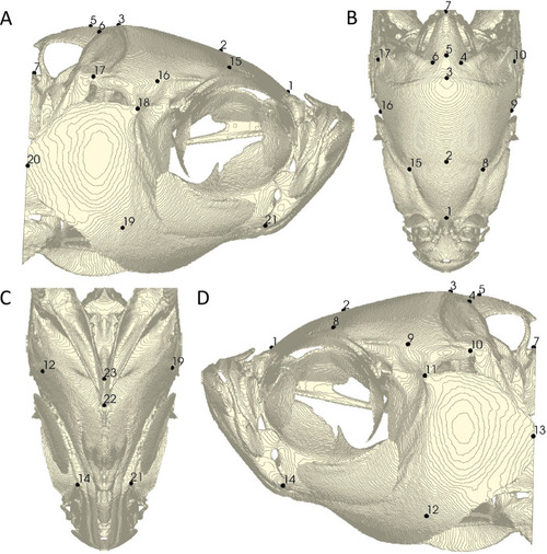
Gold standard of 23 manual landmarks. Landmark placement represents the average location of two independent landmark placements by the same author. Right lateral (A), dorsal (B), ventral (C), and left lateral (D) views of the atlas mesh are shown. Landmark definitions can be found in Table 3.

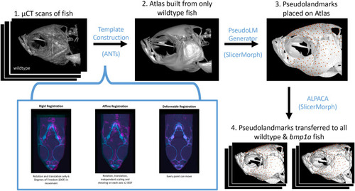
Pipeline for atlas building, pseudo-landmark generation, and transferring pseudo-landmarks to individual fish. Blue text notes the software used between each step. (1) Starting with µCT scans of wild-type fish, ANTs uses a series of rigid, affine, and deformable registrations to create an average image, or (2) Atlas. The PseudoLMGenerator tool in SlicerMorph was used to (3) place 372 pseudo-landmarks on the atlas. The ALPACA tool in SlicerMorph was used to (4) transfer points from the atlas to wild-type and bmp1a fish for comparisons between groups.

ZFIN is incorporating published figure images and captions as part of an ongoing project. Figures from some publications have not yet been curated, or are not available for display because of copyright restrictions.