(A) in situ hybridization chain reaction (HCR) was used to stain for msgn1 (yellow) and tbx6 (red), markers of the posterior and anterior PSM, respectively, from the 16 somite-stage to the end of somitogenesis. Nuclei were stained with DAPI (grey). (B) 2D contours (yellow outlines, left image) were manually drawn around the PSM at regular z-slices, up to the midline, to generate 3D surface reconstructions of the PSM (cyan, right image) and the nascent (i.e. most recently-formed) somite (Fig S1D) at each stage. (C) DAPI signal was isolated from each surface to show only nuclei in that tissue. (D) Spots were generated, marking the centre of each isolated nucleus (shown in slice view (left image) and 3D view (other images)), and providing cell number information. (E-J) The length, cell number, and volume of the PSM (E-G) and of each somite at its time of formation (H-J) was measured for a range of stages. Each point represents the PSM/nascent somite of a single embryo (n = 15 embryos for length data, n = 11 embryos for cell number data and n = 26 embryos for volume data). Possible trendline equations for each measurement were calculated in R, and AIC was used to determine the best statistical model (linear vs exponential). Solid trendlines (blue, PSM) indicate genuine change of one tissue over time, whereas dotted trendlines (red, nascent somites) indicate a trend based on separate tissues. The trendline equations are as follows (where x is somite stage): PSM length (E) = -14.1x + 155 (R² = 0.97); PSM cell number (F) = -139x + 4,620 (R² = 0.95); PSM volume (G) = 16,700,000e^-0.159x (R² = 0.98); Nascent somite length (H) = -1.58x + 75 (R² = 0.72); Nascent somite cell number (I) = -15.1x + 525 (R² = 0.83); Nascent somite volume (J) = 1,630,000e^-0.151x (R² = 0.94). (K-M) The above trendline equations were used to calculate how the length (K), cell number (L), and volume (M) of the paraxial mesoderm changed over time, by summing (for each stage) the current nascent somite and all previous nascent somite values to the current PSM value.

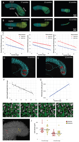
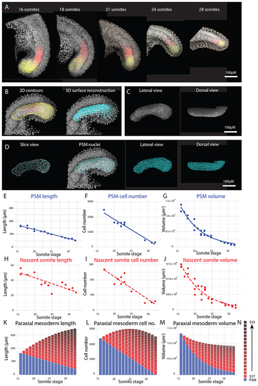
(A-B) Height (DV axis) (A) and width (ML axis) (B) measurements were taken of the posterior PSM (yellow line), anterior PSM (red line), and nascent somite (not shown) from the 16 somite-stage to the end of somitogenesis. (C) All height and width measurements show a decrease over the course of somitogenesis (n = 15 embryos). Solid trendlines indicate genuine change of one tissue (PSM) over time, whereas dotted trendlines indicate a trend based on separate tissues (nascent somites). The trendline equations are as follows (where x is somite stage): posterior PSM height = -3.88x + 172 (R² = 0.84); posterior PSM width = -2.2x + 91.6 (R² = 0.77); anterior PSM height = -1.62x + 98.7 (R² = 0.58); anterior PSM width = -2.45x + 93.1 (R² = 0.91); nascent somite height = -2.85x + 127 (R² = 0.89); nascent somite width = -2.12x + 82.4 (R² = 0.79). (D, E) Using a photoconvertible protein, dorsoventral stripes of cells in the PSM were photolabelled (red) and imaged over four somite-stages (n = 7 embryos). (F) The height and length of each label at the beginning and end of imaging was measured, along with the initial distance of the label from the posterior end of the PSM. These measurements were used to calculate a length/height ratio fold change over time, which is plotted over initial position AP position of the label (normalized from 0 to 1 between embryos, with 0 being the posterior end and 1 being the nascent somite posterior boundary). Dotted trendline equation: y = -2.17x + 2.87 (R² = 0.78). (G) PSM density (cell number divided by tissue volume) increases over the course of somitogenesis. Trendline equation: y = 0.000121x + 0.000187 (R² = 0.85). (H) Phalloidin-stained (green) tails of 18 somite-stage and 26 somite-stage embryos were used to measure cell volumes, by drawing contours around the cell membrane at every z-slice (z-interval: 1 μm). This was done for 5 randomly selected posterior cells and 5 randomly selected anterior cells per embryo (n = 10 embryos). (I) 3D reconstructions of posterior (yellow) and anterior (red) PSM cells, generated from manually-drawn contours. (J) Dotplot showing cell volumes between regions and between stages. Cell volumes were obtained from 3D cell reconstructions. Cell volumes are not significantly different between regions (t = -0.36, p = 0.72) but are significantly different between stages (t = 6.39, p < 0.001). The black dotted line represents the mean cell volume for each stage.

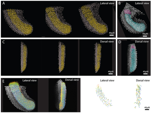
Tracks were generated of the whole tailbud and all non-paraxial mesoderm tracks were then manually removed. Paraxial mesoderm (PM) tracks (yellow spots) and non-paraxial mesoderm tracks (grey spots) shown at 0, 1, and 2 hours after imaging. (B) PM spots reconstructions (cyan: PSM & pink: nascent somite) from a similar-stage HCR image is shown for comparison/validation of selection accuracy. (C, D) The same images as above, but from a dorsal view: anterior is top, medial is left. (E) All PM tracks of full movie (colour-coded by time) superimposed over first frame image, shown for lateral and dorsal views (left images), and a sub-set of tracks shown in isolation, for lateral and dorsal views (right images).

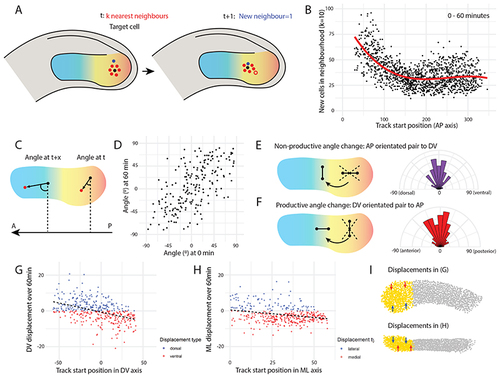
(A) Analysis of neighbour exchanges. For each paraxial mesoderm cell (black), a neighbourhood was specified as a given number (k) of nearest neighbours (red cells). After a given time interval, the number of new cells (blue) that entered the target cell’s neighbourhood was calculated. In this example, one new cell joins the neighbourhood (k = 6) over time, with the cell that is no longer in the neighbourhood shown in red outline. (B) The number of new cells entering each target cell’s neighbourhood (k = 10) over 60 min is plotted against the initial AP position of the target cell, with 0 being the posterior end of the tail, and ~ 300 being the anterior-most cells. Each point represents a single cell (n = 1,348 cells from one embryo). The results show that more cell mixing occurs in the posterior PSM (C) Analysis of neighbour angle changes. For each posterior PSM cell (black), the angle between the vector to the nearest neighbour (red) and the AP axis was calculated at the initial timepoint (t). After a given time interval (t + x), the same vector angle was calculated between the two cells (regardless of whether they were still neighbours). 0°: cells lie perpendicular to the AP axis. 90°/-90°: cells lie parallel to the AP axis. An angle change from 0° to 90°/-90° would indicate strong directional intercalation of neighbouring cells. (D) Measured neighbour angle changes are shown for 60 min. Each point represents a cell pair (n = 201 cell pairs from one embryo), with the x-axis value providing the initial vector angle and the y-axis value providing the vector angle after 60 min. (E-F) Comparing the distribution of non-productive vs productive angle changes. (E) Those neighbour pairs that initially lay parallel to the AP axis (DV angle > -45° & < 45°) were selected, and the distribution of DV angle changes over 60 min is shown on the right. (F) Those neighbour pairs that initially lay perpendicular to the AP axis (AP angle > -45° & < 45°) were selected, and the distribution of AP angle changes over 60 min is shown on the right. The distributions of angle changes are not significantly different (Two-sample Kolmogorov-Smirnov test: D = 0.069652, p = 0.7141), suggesting that directional intercalation is not occurring. (G-I) Analysis of posterior PSM cell displacements (n = 1,161 cell tracks from one embryo). (G) Strong DV axis convergence over 120 min: dorsal cells (x > 0) move ventrally (y < 0, red) and ventral cells (x < 0) move dorsally (y > 0, blue). y = -0.1x − 0.67 (R² = 0.2). (H) Weak ML axis convergence over 120 min: lateral cells (high x) move medially (y < 0, red) and medial cells (low x) move laterally (y > 0, blue). y = -0.08x + 0.45 (R² = 0.08). (I) Schematic summarising displacements of posterior PSM cells (not to scale). Top view is lateral, showing DV convergence. Bottom view is dorsal, showing ML convergence.