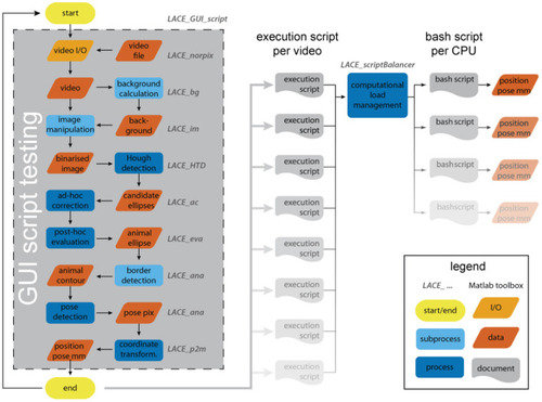
The analysis flow of LACE. The user interacts with most toolboxes through a graphical user interface (GUI). The GUI results in an execution script that holds all information and file positions to run an analysis on the entire video. By testing the script inside the GUI, the system is able to calculate the analysis duration, which is used in the computational load management. The bash scripts can be run over night.

Image Manipulation. (A) Raw footage of a zebrafish video. The animal is depicted on the right border of the area. (B) Respective difference image. (C) Binarised image with a threshold of 0.25 (D) Binarised image after erosion and dilatation (image morphology).

These are illustrations of five standard problems LACE_ac toolbox can automatically detect and solve. Problem 1 and 2 are superfluous detections of either the same animal (Problem 1) or other contrast areas in the video frame like shadows (Problem 2). Both are solved by deleting the detection with the lower quality rating. Problem 4 results from one of the detection ellipses not passing all criteria (size, eccentricity, last position) and is solved by taking the detection with the highest quality from the sub-threshold detection list. Problem 5 to 7 are all due to a miss-detection in which two or more animals are lumped together, because of their proximity. These are mainly solved by deleting detections that are too large and choosing from the sub-threshold detection list (Problems 5 and 6) or by splitting up the chain in animal long regions (Problem 7).

Schematic overview of the pseudo skeleton calculation. The figure illustrates the general procedure used to derive a pseudo-skeleton, therefore all vertices, contours, etc. are schematic drawings and not based on data or results of the algorithms. The pose detection uses the center of the ellipse detected by LACE_HTD toolbox as the center for a simple contour detection (solid orange line) via Canny's edge detector. One hundred evenly spaced pixel-coordinates (translucent orange dots) on the contour are chosen. Note that these contour-coordinates are not evenly spaced in the schematic drawing. These contour-coordinates are used as seeding coordinates for Voronoi cells (teal colored lines and dots). A Voronoi cell encompasses all space that is closer to its contour coordinate than to the other contour coordinates. Each cells is enclosed by a number of edges. The Voronoi calculation also generates edges of the Voronoi cells outside the contour of the animal, which are ignored in the algorithm and therefore not drawn here. These Voronoi-edges (teal lines) are represented by their vertices (teal dots). The algorithm selects the vertices that are inside the animal's contour for further computation. Those central Voronoi-edge vertices are now used in Dijkstra's path algorithm to select (teal dots with orange border) the central line along the anteroposterior-axis (dashed orange line).

A histogram of the correction frequency per frame for 1,318 different zebrafish video. 1,176 videos needed no correction at all. In 107 videos, less than 5% of the frames were corrected. Note that the counts are depicted on a logarithmic scale. Above the histogram bars, a rug plot (similar to a scatter plot) of the occurrences is given. Each vertical marker represents a video at the given correction frequency on the x-axis.

Quantification of body peristaltic contractions of freely crawling Drosophila larvae. The results of two trajectories traced with LACE are shown in (A–C): (A) the curvature, (B) eccentricity, and (C) normalized body length of a wild-type (CantonS) larva (orange) and a nan^36a mutant larva (blue). The curve finder (A) detects portions of the video where turning is detected. The turns appear as gray shaded areas (point 2 for CantonS and points 2 and 3 for nan^36a). The white background shows peristaltic contractions during forward crawling (points 1 and 3 for CantonS and 1 for nan^36a). Above (wildtype) and below (nan^36a) still frames from the corresponding times (1,2,3) are depicted. The pseudo-skeleton is superimposed as a light blue line, the contour of the animal is shown as solid green line, the central contour as a dashed green line, and the gut as a red line. Both markers (gut, central contour) were not used in this analysis. In (D) the contraction amplitude is quantified for wildtype, w¹¹¹⁸ , nan^36a and iav¹ mutant larvae. The nan^36a and iav¹ mutants have significantly lower body contraction amplitudes compared to wildtype CantonS and w¹¹¹⁸. The dataset consists of 30 wildtype larvae (CantonS), 26 w¹¹¹⁸ larvae, 8 nan^36a larvae, and 12 iav¹ larvae. Statistical significance was tested with Fisher's permutation test on different medians. ***p < 0.001, **p < 0.01.

An example trajectory of an adult zebrafish traced with LACE. (A) Top view of the trajectory. The body's pseudo-skeleton is plotted as a line every 50 ms. Time is color coded by the color-bar. Three segments of the trajectory were chosen for a close up representation in B. 1 and 3 depicts fast turns and 2 shows a phase of undulatory body wave propulsion. (B) Enlarged view of the three segments from A. The pseudo-skeleton is now plotted every 5 ms. Time is encoded by the color bar. (C–E) show quantification of the trajectory over time. The gray areas mark the time in which the 3 segments (subplot B) occurred. (C) Thrust velocity in m*s⁻¹. (D) is a YY-plot. The dark blue axis presents the yaw angle in degrees (shown in the same color). The light blue axis shows the yaw velocity in °*s⁻¹ (shown in the same color). (E) depicts the mean angle of the pseudo-skeleton parts to each other. If the pseudo-skeleton is a perfect line, the angle is 180° and should decrease the more the skeleton is bent.

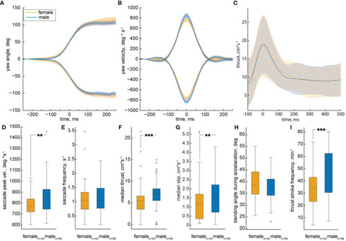
Analysis of multiple trajectories by female and male zebrafish during motivated trials. The median yaw angle (A) and velocity (B) of turn triggered averages plotted against time. The solid line represents the median of all individuals, shaded areas represents 95% confidence interval. Females are represented by the orange color, males by a blue color. Yaw to the left/right is indicated by positive/ negative numbers, respectively. The yaw angle over time is equal between male and female. Males exhibit higher maximal velocities compared to females. (C) The triggered average of all spikes of propulsion is plotted against time. The shaded area represents standard deviation from the mean. There is no significant difference in the propulsion and gliding motion of male and female. (D–I) show the quantification of different types of locomotion in the form of box plots. The black line represents the median of all individuals, the box displays the upper and lower quartile, the whiskers denote 1.5 times the interquartile distance and the plus-signs mark the outliers. Color is coded as in A. (D,E) The saccadic peak velocity of females as compared to males is significantly lower, while there is no significant difference in the saccade frequency between the two. (F,G) The median thrust and slip velocities of male fish are significantly higher as compared to the females. (H) There is no difference in the body-bending angle during acceleration. (I) There is a significant decrease in the frequency of thrust stroke of females as compared to males. The data set consists of 59 males and 43 females. Statistic significance was tested with Fisher's exact permutation test on different medians. ***p < 0.001, **p < 0.01.