Figure 1. Methodology overview. (A) Image slice 51 (150 μm from the dorsal plane, shown in F) from WT zebrafish embryo time-lapse set at 24 hpf obtained via multiphoton microscopy. FB, forebrain; MB, midbrain; HB, hindbrain; MHB, midbrain-hindbrain boundary. Scale bars, 50 μm. (B) Binary filtering. (C) Image after noise removal and region extraction; colors are inverted and intensity is adjusted for presentation. (D) Initial 2D BOC (linearly connected red spheres). Note the rough outline. (E) After refinement, contour is smoother. Insets correspond to solid and dashed rectangles in (C). (F) Refined 3D mesh. There are 56 slices, imaged 3 μm apart. The z dimension is exaggerated to show the 2D BOC of slices 6, 23, 36, and 51. (G) Mesh in (F) viewed from the ventral side. Color scale from 1 to 56 corresponds to slice number from dorsal to ventral planes. Inset is view of the rectangle looking into the mesh from the top left corner. View is rotated 130° counterclockwise about the y axis. Part of the outer mesh is hidden in the viewing plane to reveal the inner mesh. (H) 2D BOC of slice 51 after stage 3 refinement. Note the further refined regions compared to (E). BOC is overlaid onto the original image in (A) for comparison.

Figure 2. Pixel noise removal. (A–C) Area-based noise removal of slice 36. (B) Two areas after binary thresholding and inverting. (C) After removing holes and debris using a 20-pixel area cutoff. The same area size cutoff was used for all slices. (D–F) Rank-based cluster removal of slice 45. (E) After binary thresholding and inverting. Four largest clusters are ranked by size (1 is the largest and includes all the background in this slice). Inset shows enlarged view of the rectangle in (D); the cluster ranked number 4 is circled in blue. Holes and debris are marked by red circles, as in (B). (F) Binary mage after rank-based noise removal. The three largest clusters were kept.

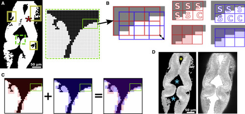
Figure 3. Contiguous region extraction. (A) Binary thresholded image from Fig. 1 B. Solid rectangles mark irregular protrusions. Inset is a magnified view of the area marked by the dashed rectangle. A star marks the point for initiating region extraction. (B) Positions of two 3 × 3 pixel grids for the area within the solid rectangle in the inset of (A). Black was changed to gray for presentation. Double-headed arrow denotes the diagonal shift of grids (additional two grid shifts are not shown for clarity). Panels on the right show labeling each 3 × 3 window based on the intensity of pixels it contains. Checked windows (labeled “C”) are set to 255 intensity, and the sealed windows (labeled “S”) are filled with the background intensity (represented by semitransparent red or blue). (C) AND operation of the extracted foreground from two grid variations. Because red and blue represent the background, pixels where they overlap are set to 0, and pixels for which only one color is present are not changed. (D) Ventricle extraction using a 2 × 2 pixel window. The left panel is the filtered grayscale image used for ventricle extraction; stars mark the points for initiating ventricle extraction. The right panel shows the extracted ventricle (area filled in white) overlaid onto the original image for comparison.

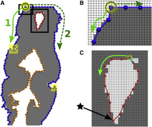
Figure 4. Assign beads and bonds. (A) BOC from Fig. 1 D. Individual chains are colored differently. Solid and dashed arrows (paths 1 and 2) denote counterclockwise and clockwise search directions along the bead boundary from the arbitrarily chosen seed bead (circled) to construct the outer chain. (B and C) Zoomed-in views of the rectangles in (A). One grid window represents one pixel. Beads and bonds are added as new edges meet the bond length cutoff b₀. Beads are assigned at pixel corners. (C) For boundary forming a closed contour, only one search direction is needed. The last bond added to close the contour is marked in cyan. Note that the sharp bend marked by a star is retained after smoothing (cf. Fig. S2).

Figure 5. Close mesh holes. (A) z-bond assignment. Mesh from Fig. 1 before refinement. Slice numbering follows Fig. 1 F. Mesh elements are labeled. Holes and pentagons of slices 5–8 are shown. Mesh after first (B) and second iterations (C) of the hole closing procedure and z-bond updates is shown. Added beads, added z-bonds, and new distance-based z-bonds pertaining to the holes in (A) are marked. Inset of (C) is zoomed view of area in the red rectangle. z-bonds marked by X were removed after the procedure to limit z-bonds to one per bead for each neighboring slice. (D) Mesh after depressing protrusions (see Fig. 6 for further detail). Note the lack of holes. (E) Mesh after final refinement steps (smoothen BOC and equalize bond length). Note decrease in the number and size of pentagons.

Figure 6. Depress mesh protrusions. (A) Mesh from Fig. 1 G colored by slice. Autofluorescence image below and in all panels corresponds to slice 51. Before (B and E) and after (D and F) mesh refinement images are shown. Insets are side views for the rectangles. Protruding beads are marked in blue. (B) Intervening beads are marked with blue squares. (C) Depressing the protrusion on slice 50 of (B) (purple highlight) using guiding points (black) on the line between the flanking beads (purple). Chain before smoothing the protrusion is shown in orange. (E) A protruding segment on slice 51 is highlighted in purple. (F) During final refinement, some beads were deleted for the equalize bond length procedure. Also see Fig. S3.

Figure 7. 3D models of images from live zebrafish embryos. WT embryos are at 20 (A and C) and 27.5 hpf (B). Mutant ace embryos are at 20.5 (D and F) and 27.5 hpf (E). For each set, the BOC of slice 35 is overlaid on the respective autofluorescence image. Mesh color scale corresponds to slice number from dorsal to ventral planes. For ace, only slices 18–42 are shown for clarity. Surface and normal vectors are shown in yellow for slices 47–50 of the WT (C) and 35–38 of the ace embryos (F). Normal vectors (arrows) point to the outside of the neuroepithelium. Fig. S4 shows models for other time points.

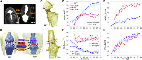
Figure 8. Measuring phenotype characteristics. (A) Extracted ventricle (solid white) from one slice of WT and ace embryos at 25 hpf. (B) 3D rendering of extracted ventricle images (blue) and embryo outline (yellow) visualized using UCSF Chimera (20). Renderings were manually oriented such that the dorsal side is facing out of the page. Measured structures are labeled. (C) 3D meshes of WT and ace embryo ventricles. Measured widths are colored in the same way as in (B). Positions marked by spheres are automatically located. MHB positions are denoted by small red spheres. Larger spheres mark the ventricles and MHB constriction. The number next to each sphere corresponds to the slice on which the sphere is located. See Fig. S5 for a detailed illustration of the automated measurement procedure. (D–G) Plots comparing voxel-based manual measurements (thick solid lines) and automated BOC-based (dashed) measurements for the two phenotypes. Manual measurements of MHB_bend (F) were taken for the right side only. BOC-based MHB_bend is measured between the vectors formed from the MHB constriction to the mesencephalic ventricle position and from the MHB constriction to the rhombencephalic ventricle position on each respective side. Error bars represent standard deviation of five manual measurements. Some error bars may be covered by marker symbols.

Figure 9. 3D BOC of human fetal brain. The cortex (slices colored based on color scale) and ventricles (yellow) are modeled at three gestational ages (weeks 28, 33, and 37). Ventral and slanted views of each structure are shown. Bottom row shows sample input image slices with BOC overlaid on the merged images of the cortex and ventricles (green BOC) for each respective time point. Normal vectors denoting the orientation of the constructed surface between slices 66 and 67 are shown. Surface curvature measurements are in Fig. S6.

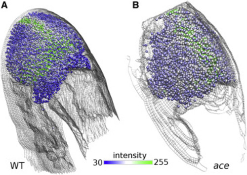
Figure 10. Combining models from two imaging channels. Spatial distribution of wnt1 expression from the GFP channel autofluorescence image over BOC of WT (A) and ace embryos at 27.5 hpf (B). One bead represents a 6 × 6 pixel area. Bead color represents the intensity of the wnt1 reporter fluorescence. Beads are not assigned to areas with pixel intensity below 30.