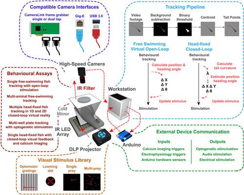
Overview of the behavioral feedback system. The behavioral feedback hardware consists of modular components based on a previous design⁵. High-speed cameras convey live video of behaving larval zebrafish to a workstation, which tracks the behavior of the fish and generates output signals to an external device to provide sensory stimulation. The workstation processes incoming video frames with BonZeb's customizable tracking pipeline. This pipeline transforms behavioral data into virtual open-loop stimulation for free-swimming fish or closed-loop stimulation for head-fixed fish. BonZeb can interface with Arduino boards, display devices, data acquisition boards, etc., for receiving or sending data. BonZeb also includes a library of common visual stimuli for closed-loop and open-loop visual stimulation. Components of the behavioral feedback system are not to scale.

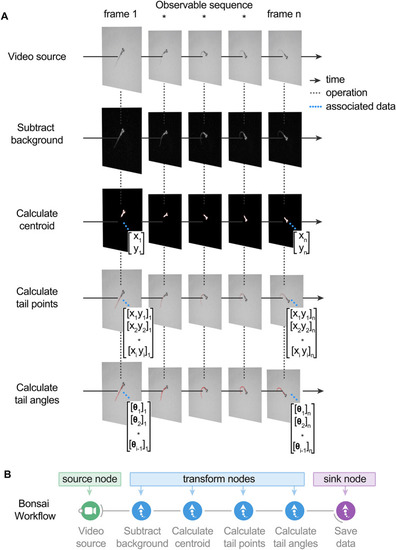
BonZeb inherits Bonsai's reactive architecture for processing data streams. (A) A video

source node generates images over time. The video source can either be a continuous stream of images from an online camera device or a previously acquired video with a fixed number of frames. A series of transformation nodes are then applied to the original source sequence. Each transformation node performs an operation on the upstream observable sequence that is then passed to downstream nodes. A typical pipeline consists of background subtraction, centroid calculation, tail point calculation, and finally, tail angle calculation. Nodes have a unique set of visualizers that provide the node’s output at each step. Each node has a set of properties associated with the output, such as a single coordinate, an array of coordinates, or an array of angles, which can be used for more sophisticated pipelines. (B) Bonsai workflow implementation of the above data processing pipeline. An additional node is attached at the end of the workflow to save the tail angles data to a csv file on disk. There are 4 different general classifications of nodes in Bonsai. Source nodes (green) generate new observable sequences and do not require inputs from upstream nodes. Transform nodes (blue) perform an operation on the elements of an upstream observable sequence to produce a new observable sequence that can be subscribed to by downstream nodes. Sink nodes (purple) perform side operations with the elements of the data stream, such as saving data to disk or triggering an external device. Sink nodes then pass along the upstream observable sequence to subscribed downstream nodes without modifying any of the elements of the upstream observable sequence. Combinator nodes (not shown here) are important for combining sequences and become crucial for more complex pipelines (see online manual for examples).

Free-swimming open-loop behavior. Individual freely-swimming zebrafish larva were presented with virtual open-loop visual stimuli while multiple behavioral metrics were recorded (332 Hz). The curvature along 14 tail segments, from the most rostral portion of the tail at the tail base to the most caudal portion of the tail at the tail tip, were calculated and averaged into 4 consecutive bins (cyan to magenta). The angle of the left (red) and right eye (green), the cumulative heading angle (yellow), the visual stimulus angle (black), tail beat frequency (orange), peak amplitudes (navy blue), and bout detection (gray) are displayed. (A) A looming dot stimulus (predator avoidance) produced a rapid escape turn followed by a burst swim and a marked divergence of the eyes (arrow). The location of the looming stimulus was fixed with respect to the heading direction and centroid position of the larvae such that the visual angle of the stimulus increased exponentially to a fixed size of the visual field. (B) During optomotor swimming, the direction of the OMR stimulus was fixed to the heading direction of the larvae and the point at which the OMR stimulus pivoted was fixed to the larva’s centroid. In this example, the OMR stimulus traversed 90° to the left of the heading direction of the fish, which consistently drove the fish to produce routine turns. (C) A small white dot on a black background was presented to larvae from below to create virtual prey stimuli. In this example, the prey stimulus moved along an arc with a fixed radius from the centroid. The velocity of the dot along the arc was defined by a sinusoidal function which reached a maximum of 100°/s directly in front of the larvae and reached a minimum of 0°/s at 60° to the left and to the right of the heading direction. Larvae displayed characteristic hunting behavior towards this stimulus by producing J-turns when the stimulus was presented to the lateral parts of the visual field and slow, approach swims when the stimulus was presented in the frontal field. These hunting episodes were also characterized by convergence of the eyes throughout the hunting episode (arrow). Images of larvae in (A–C) were adjusted so they stand out against the stimulus background.

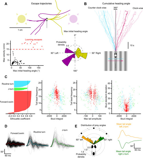
Visual stimulation drives specific behavioral kinematics. (A) Escape trajectories in the virtual open-loop looming dot assay when the looming dot was presented from the left (yellow) and from the right (magenta). Bottom left: max velocity (cm/s) with respect to the max initial heading angle (°) plotted for each bout. Bouts classified as escapes are colored red. Dashed red line represents the threshold value applied to the max velocity to select escape responses. Bottom right: probability density distribution for the max initial heading angle. (B) Cumulative heading angle over time in response to leftward (blue) and rightward (red) OMR stimulation. Spurious heading angle changes produced by fish interactions with the shallow edges of the watch glass have been removed. Rapid heading changes in the mean traces are due to the termination of shorter trials. (C) Hierarchical clustering applied to bouts in response to virtual open-loop prey stimulation. Four kinematics parameters were calculated for each bout (mean tail beat frequency, bout integral, max tail amplitude, bout standard deviation). Left: silhouette plot showing the results of hierarchical clustering with 3 clusters. Dotted line represents silhouette index. Middle-left to right: kinematic parameters plotted for each bout color-coded by cluster. (D) Black lines: tail angle over time for every bout in each cluster. Colored lines represent the mean tail angle over time across all bouts in each cluster. Results from (C,D) were used to identify the three clusters as forward swims (red), routine turns (blue), and J-turns (green). (E) Bouts in the J-turn cluster were separated into left-biased and right-biased swims. Left: probability density distribution of prey yaw angles at the start of left-biased and right-biased swims in the J-turn cluster. Right: mean tail angle over time for left (yellow) and right (green) J-turns.

Multi-animal tracking during OMR and prey capture. (A) The position and tail curvature of 12 larvae tracked (332 Hz) during the presentation of an OMR stimulus. The direction of the OMR stimulus changed to traverse leftward or rightward depending on whether the center of mass of the group crossed into the rightmost quarter or leftmost quarter of the arena, respectively. Trajectories are individually color coded by fish and shaded by time. The tail curvature for each fish is represented as the average of the 3 most caudal tail segments. Post processing of the tail curvature data revealed sections of the data when fish physically contacted each other (red highlighted regions). The tail tracking results surrounding these encounters decreased in accuracy and occasionally produced tracking errors (arrow). (B) Freely swimming larvae in a group of 6 were tracked and presented with multi-prey stimuli projected from below. Virtual prey were programmed to produce paramecia-like behavior, defined as periods of forward movement, brief pauses, and changes in orientation. The linear velocity, distance, length of pause, angular velocity, and orientation were varied for each virtual prey. Larvae produced distinct J-turns in response to virtual prey (* = manually identified J-turn).

One-dimensional head-fixed closed-loop OMR. The tail of a head-fixed fish was tracked (332 Hz) while presenting a closed-loop OMR stimulus with varying feedback gain values. (A) Example bouts taken for each gain value for a single fish. Fish were tested on 3 different gain values. Left: gain 0.5. Middle: gain 1.0. Right: gain 1.5. The stimulus velocity (black), tail angle (red), and tail beat frequency (orange) were recorded continuously throughout the experiment. The stimulus velocity changed in proportion to the swim vigor multiplied by the gain factor. Dotted lines indicate baseline value of 0. (B) An example of a single fish showing the tail beat frequency across trials. Left: tail beat frequency sorted by trial number. Right: same data as left with tail beat frequency sorted by gain. (C) Bout kinematics plotted as a function of gain factor.

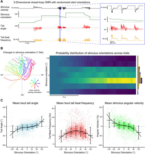
Multi-animal two-dimensional closed-loop OMR. The tails of four head-fixed fish were tracked (332 Hz) while each fish was presented with a two-dimensional closed-loop OMR stimulus. (A) Data collected for each fish included the stimulus velocity (black), stimulus orientation (green), tail angle (red) and tail beat frequency (orange). The stimulus velocity changed in proportion to the tail beat frequency and current stimulus orientation. The stimulus orientation changed with the tail angle. Trials were 30 s long and were preceded by a 1-min rest period where only the stimulus velocity and stimulus orientation data were recorded. At the end of each trial, the orientation of the stimulus was reset to one of the 8 randomized start orientations. (B) Stimulus orientation over time. Left radial plot: stimulus orientation is plotted for all trials for a single fish. Trials are color-coded based on initial starting orientation and extend outwards from the origin as a function of time. Right heatmap: normalized histograms of stimulus orientations over time across fish (n = 16). Binning was 1 s for the x-axis and 45° for the y-axis. Far right plot: histogram and kernel density estimate of the distribution of orientations at the end of trials across all fish. (C) Bout kinematics and stimulus angular velocity are plotted for each bout as a function of stimulus orientation at bout onset. Orientations were divided into 45° bins and the median and standard deviation for each bin are plotted. A polynomial function was fit to each dataset. The mean bout tail angle and mean stimulus angular velocity were fit with 3rd degree polynomials (R² = 0.223 and R² = 0.256, respectively) whereas the mean bout tail beat frequency was fit with a 2nd degree polynomial (R² = 0.05).

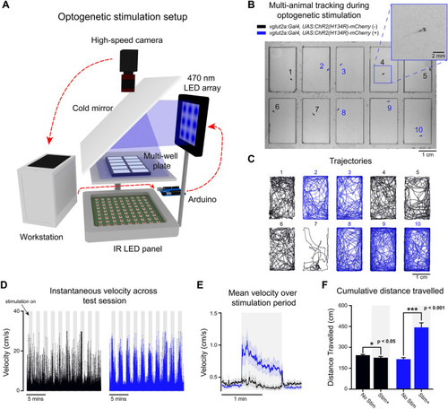
Free-swimming multi-animal tracking during optogenetic stimulation. Ten larvae were tracked simultaneously (200 Hz) in a multi-well plate while being subjected to epochs of optogenetic stimulation. (A) 3D schematic of the optogenetic stimulation setup. Live video is processed by BonZeb, which sends commands to an Arduino to generate a digital signal for triggering a 470 nm LED array (0.9 mW/mm2 at the plate). Components of the optogenetic setup are not to scale. (B) Example of a single video frame. Data are color coded based on genetic background. (C) Example of trajectories over an entire 20-min test session. (D) Instantaneous velocities for all fish plotted across the entire test session. Shaded regions represent periods when optogenetic stimulation occurred. 1-min intervals of stimulation and no stimulation repeated throughout the assay with a 30 s no stimulation period occurring at the beginning and end of the assay. Left: instantaneous velocity of control larvae (n = 15). Right: instantaneous velocity of experimental larvae (n = 15). (E) Mean instantaneous velocity averaged across all fish and all stimulation periods. Instantaneous velocity across each stimulation period was averaged for each fish and convolved with a box car filter over a 1s window. Bold line represents the mean and shaded region represents SEM. (F) Cumulative distance travelled during periods of stimulation ON (Stim +) and stimulation OFF (No stim).

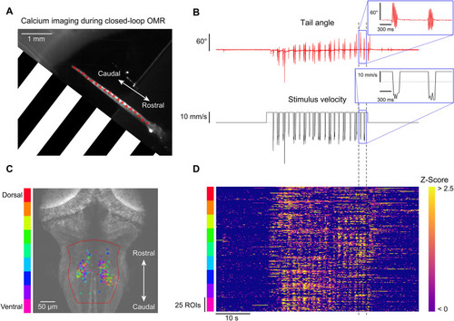
Calcium imaging during closed-loop OMR. One-dimensional closed-loop optomotor gratings were presented to a head-fixed larva while simultaneously performing fast volumetric two-photon calcium imaging. (A) Single frame obtained from the behavior camera showing the larva’s tail with the OMR stimulus represented (stimulus spatial frequency was lower than depicted; 450 Hz tracking). The OMR stimulus was presented from the side and travelled from caudal to rostral. (B) Tail angle and stimulus velocity across the entire 1-min trial. Movement of the closed-loop OMR stimulus began at 15 s and continued for 30 s. (C) Maximum intensity z-projection overlaid with neuronal ROIs found in the medial hindbrain. 25 ROIs were selected for each z-plane and color-coded by depth. Automated ROI extraction was performed throughout the region enclosed in dotted red line which helped minimize the detection of non-somatic ROIs. (D) Z-scored ROI responses across the trial.